Analog computers are based on principles completely different
from digital computers. Problem variables are represented by
electrical voltages which can vary continuously within a certain
range, usually -10 to +10 volts for a transistor-based machine.
Electronic circuit modules allow the variables to be added,
integrated (with respect to time) and multiplied by a constant.
This makes it is possible to solve a system of ordinary linear
differential equations by properly combining a number of adders,
integrators, amplifiers and potentiometers using flexible chords
and a patch panel (see the examples).
EAI 680 patch panel (detail)
Large machines like the EAI 680 also support non-linear
operations: square-rooting, arbitrary (piecewise linear) function
generation, multiplication of two variables, and comparing the
values of two variables. The last mentioned operation results in a
boolean quantity which, perhaps combined with other boolean results
(using the machine's patchable logic circuitry) can be used to
change the 'program' dynamically. For instance, the simulation of a
bouncing ball requires the solution of one differential equation
when the ball is in free fall, while another equation (describing
the forces occurring during elastic deformation) is applicable when
the ball is in ground contact. The results of the computation can
be shown graphically, in real time, on
an oscilloscope or plotter, or be digitized for being stored or
further processed by a digital computer in a hybrid system. Also
the results can be used directly for the control of some physical
process.
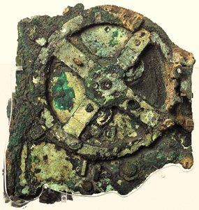
left: Antikythera, Greece 100 BC (photo wikipedia).
right: Astrolabe, Augsburg 1610. Kunstgewerbemuseum Berlin (photo E.H. Dooijes).
Early special-purpose analog computers were the ancient Antikythera, the astrolabe of the
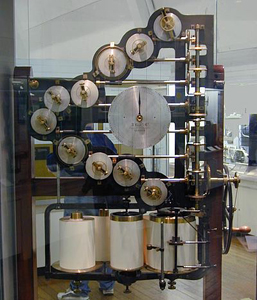
Middle Ages, the slide rule, the curvimeter and William Thomson's mechanical tide predicting machine [1]. The principle of the mechanical integrator has been described by William Thomson (Lord Kelvin) and his father James Thomson. Integration was needed in the planimeter, the harmonic analyzer, and for the solution of differential equations [3].
Thomson's mechanical tide predicting machine, Science Museum London.
General-purpose mechanical analog computers ("differential analyzers") based on Thomson's principles were built in the 1930's by Vannevar Bush (1890-1974) at MIT.
In World War II, analog computing mechanisms were of great importance for gunfire control on warships (picture below from [2]).
The paradigma of the differential analyzer strongly
influenced the architecture of the ENIAC, which was indeed designed
to replace the Bush differential analyzer for doing ballistic
calculations towards the end of World War II.
These mechanical systems were gradually replaced by electronic
machines, first with electron tubes, later with transistors. Early special-purpose examples are the TRIDAC aircraft flight simulator (1956) and the Deltar tide simulator (1961).
General-purpose analog
computers, programmed by way of patchboard wiring, and sometimes in combination with digital computers, were
heavily used until well in the 70's for applications like
automobile suspension design, chemical process simulation and
control, experimentation with 'world models', Apollo spacecraft
flight control, and many others. While the analog computer was
ideal for the fast solution of differential equations (because all
operations are effectively done in parallel), very expensive parts
and construction techniques were needed for obtaining a reasonable
accuracy of the solutions. Therefore the analog computer was
quickly superseded by the digital computer in the late 70's.
Numerous programming systems were invented to emulate the analog
computer on a digital machine: examples are CSSL (Continuous Systems Simulation Language), and TUTSIM, developed at the Technical University Twente (The Netherlands). An early version of TUTSIM is running on one of the Museum's PDP-11 computers.
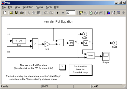
The analog computer paradigm is still alive; a graphical
programming environment for simulation like MathWorks' Simulink is built on the idea of patching together functional units, with virtual wires, for solving a given problem.
Screenshot of a Simulink program.
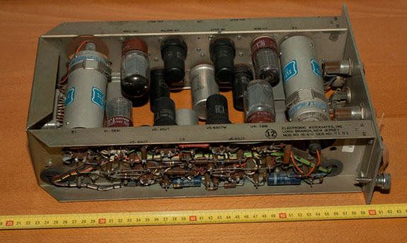
A basic building block of the analog computer is the
operational amplifier which is used in almost every
functional unit (adders, integrators, etc). It acts as the heart of
an electronic servo mechanism which (in an adder) turns the virtual
knob of the output voltage source in such a way that the output
voltage is accurately equal to the sum of the input voltages. The
operation amplifier (featuring a very high gain, high input
impedance and low output impedance) is still heavily used today -
in a miniaturized version - in a large variety of electronic
circuits among which artificial neural networks.
Dual electron-tube opamp by EAI (early 1950's).
The large aluminium cylinders are 'choppers'. The unit's weight is 4.4 kg.
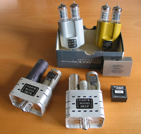
Some operational amplifiers made by Philbrick Researches.
The two smaller opamps are built from discrete transistors.
References:
[1] Wikipedia: "Tide-predicting machine".
[2] A. Svoboda: Computing mechanisms and linkages. MIT Radiation Laboratory Series no.27, McGraw-Hill 1948.
[3] W. Thomson, Treatise on Natural Philosophy Vol. 1, Cambridge 1879.
November 2014