Analog computer programming
The figure shows the set-up for the solution of a very simple second-order linear differential equation, representing the dynamics of a body moving (in one dimension) under the influence of gravity. Before the computation can be started, initial conditions (IC) must be specified. This is accomplished by charging the capacitors in both integrators to the voltages representing the zero-time velocity and position, respectively. On the patch panel a special IC input is provided for every integrator. By simply turning a console switch controlling the value of the integrating capacitors, the problem's time scale can be scaled up or down, making it suitable for plotting on a pen recorder, or for viewing on an oscilloscope. In the latter case the solution can be quickly repeated, completely automatically.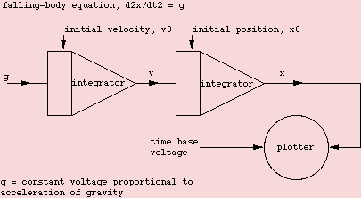
References
- MacKay and Fisher: Analogue Computing at Ultra-high Speed. Chapman & Hall (London) 1962
- Korn and Korn: Electronic Analog and Hybrid Computers. MacGraw-Hill (New-York) 1964
