

Probabilistic Causation
“Probabilistic Causation” designates a group of theories that aim to characterize the relationship between cause and effect using the tools of probability theory. The central idea behind these theories is that causes change the probabilities of their effects. This article traces developments in probabilistic causation, including recent developments in causal modeling. A variety of issues within, and objections to, probabilistic theories of causation will also be discussed.
- 1. Motivation and Preliminaries
- 2. Probability-raising Theories of Causation
- 2.1 Probability-raising and Conditional Probability
- 2.2 Screening off
- 2.3 The Common Cause Principle
- 2.4 The Fork Asymmetry
- 2.5 Simpson's Paradox and Background Contexts
- 2.6 Other Causal Relations
- 2.7 Population-relativity
- 2.8 Contextual-unanimity
- 2.9 Path-specific Causation
- 2.10 Potential Counterexamples
- 2.11 Singular and General Causation
- 3. Causal Modeling
- 4. Other Theories
- Bibliography
- Other Internet Resources
- Related Entries
This entry surveys the main approaches to characterizing causation in terms of probability. Section 1 provides some of the motivation for probabilistic approaches to causation, and addresses a few preliminary issues. Section 2 surveys theories that aim to characterize causation in terms of probability-raising. Section 3 surveys developments in causal modeling. Some of the more technical details have been relegated to the supplements. Additional probabilistic approaches to causation are surveyed in Section 4 and in the supplements.
1. Motivation and Preliminaries
In this section, we will provide some motivation for trying to understand causation in terms of probabilities, and address a couple of preliminary issues.
1.1 Problems for Regularity Theories
According to David Hume, causes are invariably followed by their effects: “We may define a cause to be an object, followed by another, and where all the objects similar to the first, are followed by objects similar to the second.” (1748, section VII.) Attempts to analyze causation in terms of invariable patterns of succession are referred to as “regularity theories” of causation. There are a number of well-known difficulties with regularity theories, and these may be used to motivate probabilistic approaches to causation. Moreover, an overview of these difficulties will help to give a sense of the kinds of problem that any adequate theory of causation would have to solve.
(i) Imperfect Regularities. The first difficulty is that most causes are not invariably followed by their effects. For example, smoking is a cause of lung cancer, even though some smokers do not develop lung cancer. Imperfect regularities may arise for two different reasons. First, they may arise because of the heterogeneity of circumstances in which the cause arises. For example, some smokers may have a genetic susceptibility to lung cancer, while others do not; some non-smokers may be exposed to other carcinogens (such as asbestos), while others are not. Second, imperfect regularities may also arise because of a failure of physical determinism. If an event is not determined to occur, then no other event can be (or be a part of) a sufficient condition for that event. The recent success of quantum mechanics—and to a lesser extent, other theories employing probability—has shaken our faith in determinism. Thus it has struck many philosophers as desirable to develop a theory of causation that does not presuppose determinism.
The central idea behind probabilistic theories of causation is that causes change the probability of their effects; an effect may still occur in the absence of a cause or fail to occur in its presence. Thus smoking is a cause of lung cancer, not because all smokers develop lung cancer, but because smokers are more likely to develop lung cancer than non-smokers. This is entirely consistent with there being some smokers who avoid lung cancer, and some non-smokers who succumb
(ii) Irrelevance. A condition that is invariably followed by some outcome may nonetheless be irrelevant to that outcome. Salt that has been hexed by a sorceror invariably dissolves when placed in water (Kyburg 1965), but hexing does not cause the salt to dissolve. Hexing does not make a difference for dissolution. Probabilistic theories of causation capture this notion of making a difference by requiring that a cause make a difference for the probability of its effect.
(iii) Asymmetry. If A causes B, then, typically, B will not also cause A. Smoking causes lung cancer, but lung cancer does not cause one to smoke. One way of enforcing the asymmetry of causation is to stipulate that causes precede their effects in time. But it would be nice if a theory of causation could provide some explanation of the directionality of causation, rather than merely stipulate it. Some proponents of probabilistic theories of causation have attempted to use the resources of probability theory to articulate a substantive account of the asymmetry of causation.
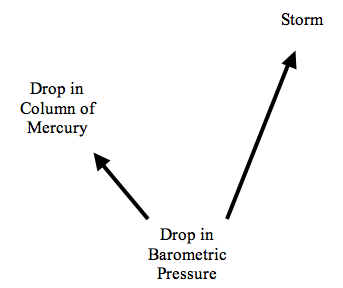
(iv) Spurious Regularities. Suppose that a cause is regularly followed by two effects. For instance, suppose that whenever the barometric pressure in a certain region drops below a certain level, two things happen. First, the height of the column of mercury in a particular barometer drops below a certain level. Shortly afterwards, a storm occurs. This situation is shown schematically in Figure 1. Then, it may well also be the case that whenever the column of mercury drops, there will be a storm. If so, a regularity theory would have to rule that the drop of the mercury column causes the storm. In fact, however, the regularity relating these two events is spurious. The ability to handle such spurious correlations is probably the greatest source of attraction for probabilistic theories of causation.
Figure 1
Further Reading: Psillos (2009). See the entries for Causation: Backward; Determinism: Causal; Hume, David; Kant and Hume on Causality; and Scientific Explanation (for discussion of the problem of irrelevance). Lewis (1973) contains a brief but clear and forceful overview of problems with regularity theories.
1.2 Probability
In this sub-section, we will review some of the basics of the mathematical theory of probability. Probability is a function, P, that assigns values between zero and one, inclusive. Usually the arguments of the function are taken to be sets, or propositions in a formal language. The formal term for these arguments is ‘events’. The domain of a probability function has the structure of a field or a Boolean algebra. This means that the domain is closed under complementation and the taking of finite unions or intersections (for sets),[1] or under negation, conjunction, and disjunction (for propositions). We will here use the notation that is appropriate for propositions, with ‘~’ representing negation, ‘&’ representing conjunction, and ‘∨’ representing disjunction. Thus if A and B are events in the domain of P, so are ~A, A&B, and A∨B. Some standard properties of probability are the following:
- If A is a contradiction, then P(A) = 0.
- If A is a tautology, then P(A) = 1.
- If P(A & B) = 0, then P(A ∨ B) = P(A) + P(B)[2]
- P(~A) = 1 − P(A).
- If A and B are in the domain of P, then A and B are probabilistically independent (with respect to P) just in case P(A & B) = P(A)P(B). A and B are probabilistically dependent or correlated otherwise.
- A random variable for probability P is a function X that takes values in the real numbers, such that for any number x, X = x is an event in the domain of P. For example, we might have a random variable T1 that takes values in {1, 2, 3, 4, 5, 6}, representing the outcome of the first toss of a die. The event T1 = 3 would represent the first toss as having outcome 3.
- The conditional probability of A given B, written
P(A | B) is standardly defined as follows:
P(A | B) = P(A & B)/P(B).
If P(B) = 0, then the ratio in the definition of conditional probability is undefined. There are, however, a variety of technical developments that will allow us to define P(A | B) when P(B) is 0. We will ignore this problem here.
Further Reading: See the entry for Probability: Interpretations of. Billingsley (1995) and Feller (1968) are two standard texts on probability theory.
1.3 Causal Relata
Causal claims have the structure ‘C causes E’. C and E are the relata of the causal claim. In probabilistic approaches to causation, causal relata are represented by events in a probability space. A number of different candidates for causal relata have been proposed. It is helpful here to distinguish two different kinds of causal claim. Singular causal claims, such as “Jill's heavy smoking during the 1990's caused her to develop lung cancer,” make reference to particular individuals, places, and times. When used in this way, cause is a success verb: the singular causal claim implies that Jill smoked heavily during the 1990's and that she developed lung cancer. The relata of singular causal claims are often taken to be events (not to be confused with events in the purely technical sense), although some authors (e.g. Mellor 2004) argue that they are facts. Since the formalism requires us to make use of negation, conjunction, and disjunction, the relata must be entities to which these operations can be meaningfully applied. We will refer to the sort of causal relation described by singular causal claims as singular causation.
General causal claims, such “smoking causes lung cancer” do not refer to particular individuals, places, or times, but only to event-types or properties. Some authors (e.g. Lewis (1973), Carroll (1991)) claim that these are just generalizations over episodes of singular causation. Others (e.g. Sober (1985), Eells (1991)) maintain that they describe causal relations among appropriately general relata such as event-types or properties. We will refer to the latter kind of causal relation as general causation.
Some authors have put forward probabilistic theories of singular causation, others have advanced probabilistic theories of general causation. When discussing various theories below, we will note which are intended as theories of singular causation, and which as theories of general causation.
For purposes of definiteness, we will use the term ‘event’ to refer to the relata of singular causation, and ‘factor’ to refer to the relata of general causation. These terms are not intended to imply a commitment to any particular view on the nature of the causal relata.
In some theories, the time at which an event occurs or a property is instantiated plays an important role. In such cases, it will be useful to include a subscript indicating the relevant time. Thus the relata might be represented by Ct and Et′. If the relata are particular events, this subscript is just a reminder; it adds no further information. For example, if the event in question is the opening ceremony of the Beijing Olympic games, the subscript ‘8/8/2008’ is not necessary to disambiguate it from other events. In the case of properties or event-types, however, such subscripts do add further information. The property ‘taking aspirin on 8/8/2008’ is distinct from the more general property of taking aspirin.
Further Reading: See the entries for Causation: The Metaphysics of; Events; Facts; Properties. Bennett (1988) is an excellent discussion of facts and events in the context of causation. See also the survey in Ehring (2009).
1.4 The Interpretation of Probability
Causal relations are normally thought to be objective features of the world. If they are to be captured in terms of probability theory, then probability assignments should represent some objective feature of the world. There are a number of attempts to interpret probabilities objectively, the most prominent being frequency interpretations and propensity interpretations. Most proponents of probabilistic theories of causation have understood probabilities in one of these two ways. Notable exceptions are Suppes (1970), who takes probability to be a feature of a model of a scientific theory; and Skyrms (1980), who understands the relevant probabilities to be the subjective probabilities of a certain kind of rational agent.
Further Reading: See the entry for Probability: Interpretations of. Galavotti (2005) and Gillies (2000) are good surveys of philosophical theories of probability.
2. Probability-raising Theories of Causation
There is a half-century long philosophical tradition of trying to analyze causation in terms of the basic idea that causes raise the probability of their effects. This section explores the major developments in this tradition.
Further Reading: Williamson (Forthcoming) is an accessible survey that covers a number of the topics in Section 2.
2.1 Probability-raising and Conditional Probability
The central idea that causes raise the probability of their effects can be expressed formally using conditional probability. C raises the probability of E just in case:
(PR1) P(E | C) > P(E).
In words, the probability that E occurs, given that C occurs, is higher than the unconditional probability that E occurs. Alternately, we might say that C raises the probability of E just in case:
(PR2) P(E | C) > P(E | ~C);
the probability that E occurs, given that C occurs, is higher than the probability that E occurs, given that C does not occur. These two formulations turn out to be equivalent in the sense that inequality PR1 will hold just in case PR2 holds.[3] Some authors (e.g. Reichenbach (1956), Suppes (1970), Cartwright (1979)) have formulated probabilistic theories of causation using inequalities like PR1, others (e.g. Skyrms (1980), Eells (1991)) have used inequalities like PR2. This difference is mostly immaterial, but for consistency we will stick with (PR2). Thus a first stab at a probabilistic theory of causation would be:
(PR) C is a cause of E just in case P(E | C) > P(E | ~C).
(PR) has some advantages over the simplest version of a regularity theory of causation (discussed in Section 1.1 above). (PR) is compatible with imperfect regularities: C may raise the probability of E even though instances of C are not invariably followed by instances of E. Moreover, (PR) addresses the problem of relevance: if C is a cause of E, then C makes a difference for the probability of E. But as it stands, (PR) does not address either the problem of asymmetry, or the problem of spurious correlations. (PR) does not address the problem of asymmetry because it follows from the definition of conditional probability that probability-raising is symmetric: P(E | C) > P(E | ~C), if and only if P(C | E) > P(C | ~E). Thus (PR) by itself cannot determine whether C is the cause of E or vice versa. (PR) also has trouble with spurious correlations. If C and E are both caused by some third factor, A, then it may be that P(E | C) > P(E | ~C) even though C does not cause E. This is the situation shown in Figure 1. Here, C is the drop in the level of mercury in a barometer, and E is the occurrence of a storm. Then we would expect that P(E | C) > P(E | ~C). In this case, atmospheric pressure is referred to as a confounding factor.
2.2 Screening off
Hans Reichenbach's The Direction of Time was published posthumously in 1956. In it, Reichenbach is concerned with the origins of temporally asymmetric phenomena, particularly the increase in entropy dictated by the second law of thermodynamics. In this work, he presents the first fully developed probabilistic theory of causation, although some of the ideas can be traced back to an earlier paper from 1925 (Reichenbach 1925).
Reichenbach introduced the terminology of “screening off” to describe a particular type of probabilistic relationship. If P(E | A & C) = P(E | C), then C is said to screen A off from E. When P(E & C) > 0, this equality is equivalent to P(A & E | C) = P(A | C)P(E | C); i.e., A and E are probabilistically independent conditional upon C.
Reichenbach recognized that there were two kinds of causal structure in which C will typically screen A off from E. The first occurs when A causes C, which in turn causes E, and there is no other route or process by which A effects E. This is shown in Figure 2.
Figure 2
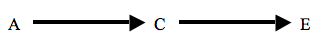
In this case, Reichenbach said that C is ‘causally between’ A and E. We might say that C is an intermediate cause between A and E, or that C is a proximate cause of E and A a distal cause of E. For example, assume (contrary to conspiracy theorists) that unprotected sex (A) causes AIDS (E) only by causing HIV infection (C). Then we would expect that among those already infected with HIV, those who became infected through unprotected sex would be no more likely to contract AIDS than those who became infected in some other way. The second type of case is where C is a common cause of A and E, depicted in Figure 1 above. Returning to our earlier example, where a drop in atmospheric pressure (C) causes both a drop in the level of mercury in a barometer (A) and a storm (E), the atmospheric pressure will screen off the barometer reading from the weather: given that that the atmospheric pressure has dropped, the reading of the barometer makes no difference for the probability of whether a storm will occur.
Reichenbach used the apparatus of screening off to address the problem of spurious correlations. In our example, while a drop in the column of mercury (A) raises the probability of a storm (E) overall, it does not raise the probability of a storm when we further condition on the atmospheric pressure. That is, if A and E are spuriously correlated, then A will be screened off from E by a common cause. More specifically, suppose that Ct and Et′ are events that occur at times t and t′ respectively, with t′ later than t. Then
(Reich) Ct is a cause of Et′ if and only if:
- P(Et′ | Ct) > P(Et′ | ~Ct); and
- There is no further event Bt″, occurring at a time t″ earlier than or simultaneously with t, that screens Et′ off from Ct.[4]
Note the restriction of t″ to times earlier than or simultaneously with the occurrence of Ct. That is because causal intermediates between Ct and Et′ will screen Ct off from Et″. In such cases we still want to say that Ct is a cause of Et′, albeit a distal or indirect cause.
Suppes (1970) independently offered essentially the same definition of causation. Interestingly, Suppes' motivation for the no-screening-off condition is substantially different from Reichenbach's. See the supplementary document:
Suppes' Motivation for the No-screening-off Condition
Suppes extended the framework in a number of directions. While Reichenbach was interested in probabilistic causation primarily in connection with issues that arise within the foundations of statistical mechanics, Suppes was interested in defining causation within the framework of probabilistic models of scientific theories. For example, Suppes offers an extended discussion of causation in the context of psychological models of learning.
In both Reichenbach's and Suppes' theories, the causal relata are events that occur at particular times, hence these theories should be understood as theories of singular causation.
Further Reading: See the entry for Reichenbach, Hans.
2.3 The Common Cause Principle
Reichenbach formulated a principle he dubbed the ‘Common Cause Principle’ (CCP). Suppose that events A and B are positively correlated, i.e., that
- P(A & B) > P(A)P(B).
But suppose that neither A nor B is a cause of the other. Then Reichenbach maintained that there will be a common cause, C, of A and B, satisfying the following conditions:
- 0 < P(C) < 1
- P(A & B | C) = P(A | C)P(B | C)
- P(A & B | ~C) = P(A | ~C)P(B | ~C)
- P(A | C) > P(A | ~C)
- P(B | C) > P(B | ~C).
When events A, B, and C satisfy these conditions, they are said to form a conjunctive fork. 5 and 6 follow from C's being a cause of A and a cause of B. Conditions 2 and 3 stipulate that C and not-C screen off A from B. Conditions 2 through 6 entail 1.
Reichenbach says that the common cause explains the correlation between A and B. Although Reichenbach is not always clear about this, the most sensible way of understanding this is as what Hempel (1965) calls a Deductive-Statistical explanation. The probabilistic or statistical fact described in 1 is explained in terms of further probabilistic facts, captured in 2–6. The idea is that probabilistic correlations that are not the result of one event causing another are to be explained in terms of probabilistic correlations that do result from a causal relationship.
Reichenbach's CCP has engendered a number of confusions. Some of these are addressed in the supplementary document:
Common Confusions Involving the Common Cause Principle
There are a number of cases where Reichenbach's CCP is known to fail, or at least to require appropriate restrictions.
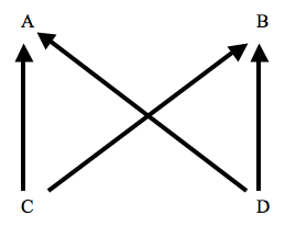
(i) If events A and B have more than one common cause, for example in the causal structure shown in Figure 3, then there will be no one common cause that screens A off from B. For example, if we condition on the common cause C in Figure 3, then A and B will still be correlated (in violation of condition 3) due to D.
Figure 3
(ii) CCP may fail if events A and B are not distinct, in the sense articulated by Lewis (1986a). For example, it may fail if A and B are logically related, or involve spatiotemporal overlap. Suppose that events E, F, and G are completely unrelated, and that they are probabilistically independent. Define A to be E & F, and B to be E & G. Now A and B will be correlated, due to the logical overlap, and there may be no cause that screens them off. Or suppose that I am throwing darts at a target, and that my aim is sufficiently bad that I am equally likely to hit any point on the target. Suppose that a and b are regions of the target that almost completely overlap. Let A be the event of the dart's landing in region a, B the dart's landing in region b. Now A and B will be correlated, and there may well be no cause that screens them off.
(iii) CCP fails for certain quantum systems involving distant correlations. For example, if we have two particles in the singlet state, and measure the spin of each in, say, the vertical direction, we will find that the probability of spin up equals the probability of spin down equals .5 for both particles. The probability that particle one is spin up while particle two is spin down is not .25 but .5, so the two measurement results are correlated. However, it can be shown that there is no (local) common cause that screens off the two measurement outcomes.
(iv) CCP may appear to fail if we use events that are too coarsely grained. Salmon (1984) gives the following example. Suppose that I am playing pool, and shooting the cue ball at the eight ball. If the cue ball hits the eight ball, the latter may or may not go into the corner pocket. But the balls are lined up in such a way that if the cue ball hits the eight ball in the right way to send it into the corner pocket, the cue ball will rebound off the eight ball in such a way as to land in the other corner pocket. Thus the events of the two balls going into the corner pockets are correlated. The events are not screened off by conditioning on the collision between the cue ball and the eight ball. However, if we condition on a more detailed specification of the angle at which the two balls collide, the probability for each ball to go into the pocket will be zero or one. In this case, the two events will perforce be independent.
(v) CCP can fail if we mix populations of different types. For example, suppose that we have a population that contains both giraffes and rhinos. Giraffes are taller than rhinos, and have better eyesight. Thus in the mixed population, height and visual acuity will be correlated, even if the developmental processes involved in the two traits are completely independent. One possible reply is that the population to which one belongs can act as a common cause. In this case, if we condition on whether an individual is a giraffe or a rhino, height and eyesight will be screened off. It's not clear, however, that population membership is the sort of thing that can properly be called a cause.
(vi) CCP may appear to fail if we collect data from time series with similar trends. Sober (2001) notes that sea levels in Venice and bread prices in London have both been steadily increasing. Therefore, the two will be correlated: higher sea levels in Venice will tend to correspond to higher bread prices in London. But the two trends (we may assume) are completely independent. It's not clear, however, that the counterexample persists when we pay sufficient attention to the relata. Recall that for Reichenbach, the causal relata are particular events that occur at specific times. Choose some particular time t, and let At and Bt be events involving the sea level in Venice and the price of bread in London at t (respectively). Now it's not clear that we can make any sense of a probability assignment in which P(At & Bt) > P(At)P(Bt). In particular, sampling sea levels and bread prices at times other than t is not an appropriate method for estimating these probabilities, since we are not sampling from a stationary distribution. (By analogy, we would not say that I had a probability of 2/3 of being over six feet tall on my third birthday, just because I have been over six feet tall on roughly two-thirds of the birthdays I have ever had.)
Further Reading: See the entries for Physics: Reichenbach's Common Cause Principle; Quantum Theory: the Einstein-Podolsky-Rosen Argument in; Reichenbach. Salmon (1984) contains an extensive discussion of conjunctive forks.
2.4 The Fork Asymmetry
Reichenbach's definition of causation, discussed in Section 2.2 above, appeals to time order: it requires that a cause occur earlier than its effect. But Reichenbach also thought that the direction from causes to effects can be identified with a pervasive statistical asymmetry. Suppose that events A and B are correlated, i.e., that P(A & B) > P(A)P(B). If there is an event C that satisfies conditions 2–6 above, then the trio ABC is said to form a conjunctive fork. If C occurs earlier than A and B, and there is no event satisfying 2 through 6 that occurs later than A and B, then ACB is said to form a conjunctive fork open to the future. Analogously, if there is a later event satisfying 2 through 6, but no earlier event, we have a conjunctive fork open to the past. If an earlier event C and a later event D both satisfy 2 through 6, then ACBD forms a closed fork. Reichenbach's proposal was that the direction from cause to effect is the direction in which open forks predominate. In our world, there are a great many forks open to the future, few or none open to the past. Reichenbach considered this asymmetry to be a macro-statistical analog of the second law of thermodynamics. See the supplementary document:
The Fork Asymmetry and the Second Law of Thermodynamics
for further discussion.
Arntzenius (1990) points out that the fork asymmetry is highly problematic in the context of classical statistical mechanics within which Reichenbach was working. Suppose that ACB forms a conjunctive fork in which C precedes A and B. Then we can evolve C forward in time deterministically to get a new event D which occurs after A and B, but stands in the same probabilistic relationship to A and B that C did. Then ACBD will form a closed fork. We may suspect that any such D will be too heterogeneous or gerrymandered to constitute an event, but there seems to be no principled reason for thinking that in all such cases, the earlier screener will be coherent enough to be a proper event, while the later screener will not be.
Further Reading: See the entry for Reichenbach. Dowe (2000), Hausman (1998), and Horwich (1987) all contain good discussions of the fork asymmetry. See also Price and Weslake (2009) for a survey of issues connected with the asymmetry of causation.
2.5 Simpson's Paradox and Background Contexts
In the Reichenbach-Suppes definition of causation, the inequality P(Et′ | Ct) > P(Et′ | ~Ct) is necessary, but not sufficient, for causation. It is not sufficient, because it may hold in cases where Ct and Et′ share a common cause. Unfortunately, common causes can also give rise to cases where this inequality is not necessary for causation either. Suppose, for example, that smoking is highly correlated with living in the country: those who live in the country are much more likely to smoke as well. Smoking is a cause of lung cancer, but suppose that city pollution is an even stronger cause of lung cancer. Then it may be that smokers are, over all, less likely to suffer from lung cancer than non-smokers. Letting C represent smoking, B living in the country, and E lung cancer, P(E | C) < P(E | ~C). Note, however, that if we conditionalize on whether one lives in the country or in the city, this inequality is reversed: P(E | C & B) > P(E | ~C & B), and P(E | C & ~B) > P(E | C & ~B). Such reversals of probabilistic inequalities are instances of “Simpson's Paradox.” This problem was pointed out by Nancy Cartwright (1979) and Brian Skyrms (1980) at about the same time.
Cartwright and Skyrms sought to rectify the problem by replacing conditions (i) and (ii) with the requirement that causes must raise the probability of their effects in various background contexts. Cartwright proposed the following definition:
(Cart) C causes E if and only if P(E | C & B) > P(E | ~C & B) for every background context B.
Skyrms proposed a slightly weaker condition: a cause must raise the probability of its effect in at least one background context, and lower it in none. A background context is a conjunction of factors. When such a conjunction of factors is conditioned on, those factors are said to be “held fixed.” To specify what the background contexts will be, then, we must specify what factors are to be held fixed. In the previous example, we saw that the true causal relevance of smoking for lung cancer was revealed when we held country living fixed, either positively (conditioning on B) or negatively (conditioning on ~B). This suggests that in evaluating the causal relevance of C for E, we need to hold fixed other causes of E, either positively or negatively. This suggestion is not entirely correct, however. Let C and E be smoking and lung cancer, respectively. Suppose D is a causal intermediary, say the presence of tar in the lungs. If C causes E exclusively via D, then D will screen C off from E: given the presence (absence) of tar in the lungs, the probability of lung cancer is not affected by whether the tar got there by smoking. Thus we will not want to hold fixed any causes of E that are themselves caused by C. Let us call the set of all factors that are causes of E, but are not caused by C, the set of independent causes of E. A background context for C and E will then be a maximal conjunction, each of whose conjuncts is either an independent cause of E, or the negation of an independent cause of E.
Note that the specification of factors that need to be held fixed appeals to causal relations. This appears to rob the theory of its status as a reductive analysis of causation. In fact, however, the issue is substantially more complex than that. The theory imposes probabilistic constraints upon possible causal relations, and there will be some sets of probability relations that are compatible with only one set of causal relations. In any event, even if there is no reduction of causation to probability, a theory detailing the systematic connections between causation and probability would still be of considerable interest.
Cartwright intended her theory as a theory of general causation, or as she put it, of ‘causal laws’. Hence the relata C and E occurring in (Cart) refer to event-types or properties, and not to events that occur at specific times. Cartwright claims that it is no longer necessary to appeal to the time order of events to distinguish causes from effects in her theory. That is because it will no longer be true in general that if C raises the probability of E in every relevant background context B, then E raise will the probability of C in every background context B′. The reason is that the construction of the background contexts ensures that the background contexts relevant to assessing C's causal relevance for E are different from those relevant to assessing E's causal relevance for C. Nonetheless, as Davis (1988) and Eells (1991) show, Cartwright's account will still sometimes rule that effects bring about their causes. Suppose that the process of human conception is indeterministic, so that conditioning upon all of the causes only serves to fix a certain probability for conception. Suppose, moreover, that conception is necessary for birth. Then conditioning upon birth will raise the probability of conception, even if all of the other causes of conception are held fixed.
Further Reading: Cartwright's theory is presented in Cartwright (1979), and further developed in Cartwright (1989). Skyrms (1980) presents a similar theory. See also the entry for Simpson's paradox.
2.6 Other Causal Relations
Cartwright defined a cause as a factor that increases the probability of its effect in every background context. But it is easy to see that there are other possible probability relations between C and E. Eells (1991) proposes the following taxonomy:
(Eells)
- C is a positive cause (or cause) of E if and only if P(E | C & B) > P(E | ~C & B) for every background context B.
- C is a negative cause of E (or C prevents E or C inhibits E) if and only if P(E | C & B) < P(E | ~C & B) for every background context B.
- C is causally neutral for E (or causally irrelevant for E) if and only if P(E | C & B) = P(E | ~C & B) for every background context B.
- C is a mixed cause (or interacting cause) of E if it is none of the above.
C is causally relevant for E if and only if it is a positive, negative, or mixed cause of E; i.e., if and only if it is not causally neutral for E.
It should be apparent that when constructing background contexts for C and E one should hold fixed not only (positive) causes of E that are independent of C, but also negative and mixed causes of E;[5] in other words, one should hold fixed all factors that are causally relevant for E, except those for which C is causally relevant. This suggests that causal relevance, rather than positive causation, is the most basic metaphysical concept.
Eells' taxonomy brings out an important distinction. It is one thing to ask whether C is causally relevant to E in some way; it is another to ask in which way C is causally relevant to E. To say that C causes E is then potentially ambiguous: it might mean that C is causally relevant to E; or it might mean that C is a positive cause of E. Probabilistic theories of causation can be used to answer both types of question.
Further Reading: Eells (1991), chapters 2 through 5.
2.7 Population-relativity
Eells (1991) claims that general causal claims must be relativized to a population. A very heterogeneous population will include a great many different background conditions, while a homogeneous population will contain few. A heterogeneous population can always be subdivided into homogeneous subpopulations. It will often happen that C is a mixed cause of E relative to a population P, while being a positive cause, negative cause, or causally neutral for E in various subpopulations of P.
Further Reading: Eells (1991), chapter 1.
2.8 Contextual-unanimity
According to both (Cart) and (Eells), a cause must raise the probability of its effect in every background context. This has been called the requirement of contextual-unanimity. Dupré (1984) has criticized this requirement. See the supplementary document:
Contextual-unanimity and Dupré's Critique
for discussion of this issue.
2.9 Path-specific Causation
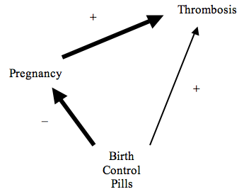
We saw in Section 2.6 above that it would be undesirable to hold fixed all of the causal factors that are intermediate between C and E, for this would hide any causal relevance of C for E. Nonetheless, it can sometimes be informative to hold fixed some causal intermediaries between C and E. As an illustration, consider a well-known example due to Germund Hesslow (1976). Consumption of birth control pills (B) is a risk factor for thrombosis (T). On the other hand, birth control pills are an effective preventer of pregnancy (P), which is in turn a powerful risk factor for thrombosis. This structure is shown in Figure 4. Overall, birth control pills lower the probability of thrombosis. Nonetheless, there seems to be a sense in which it is correct to say that birth control pills cause thrombosis. Here is what is going on: The use of birth control pills affects one's chances of suffering from thrombosis in two different ways, one ‘direct’, and one via the effect of pills on one's chances of becoming pregnant. Whether birth control pills raise or lower the probability of thrombosis overall will depend upon the relative strengths of these two routes. As it turns out, for many women, the indirect route is stronger than the direct route, so the overall effect is to prevent thrombosis. Hitchcock (2001) suggests an analogy with component forces and net forces in Newtonian physics. Birth control pill use exerts two distinct component effects upon thrombosis, one positive (causative), the other negative (preventative). The net effect is negative. The theories of Cartwright and Eells, which do not hold fixed any causal intermediates, are designed to detect net effects. However, if we hold fixed whether a woman becomes pregnant or not, we find that birth control pills increase the probability of thrombosis both among those who do become pregnant, and those who do not. By holding fixed whether or not a woman becomes pregnant, we can isolate the component effect of pills on thrombosis via the other causal pathway. More generally, we can determine the component effect of C for E along a causal pathway by holding fixed (positively or negatively) all factors that are causal intermediates between C and E that do not lie along the given the path (together with the other factors required by the theory).
Figure 4
Further Reading: Hitchcock (2001), Pearl (2001).
2.10 Potential Counterexamples
Given the basic probability-raising idea, one would expect putative counterexamples to probabilistic theories of causation to be of two basic types: cases where causes fail to raise the probabilities of their effects, and cases where non-causes raise the probabilities of non-effects. The discussion in the literature has focused primarily on the first sort of example.
(i) Probability-lowering Causes. Consider the following example, due to Deborah Rosen (reported in Suppes (1970)). A golfer badly slices a golf ball, which heads toward the rough, but then bounces off a tree and into the cup for a hole-in-one. The golfer's slice lowered the probability that the ball would wind up in the cup, yet nonetheless caused this result. One way of avoiding this problem, suggested in Hitchcock (2004a) is to make causal claims explicitly contrastive. Let S represent the golfer's slicing the ball, H her hitting a hole-in-one, and B be the appropriate background context. Now ~S is actually a disjunction of several alternatives: if the golfer hadn't sliced the ball, she might have hit the ball cleanly (S′), or missed it altogether (S″). Rather than saying that the golfer's slicing the ball caused the hole-in-one, and trying to analyze this claim by comparing P(H | S & B) and P(H | ~S & B), we can make two more precise contrastive claims. The golfer's slicing the ball, rather than missing entirely, caused the hole-in-one, as evidenced by the probabilities P(H | S & B) > P(H | S″ & B), but her slicing the ball rather than hitting it squarely did not cause the ball to go in the hole: P(H | S & B) < P(H | S′ & B). Hitchcock (1996) and Schaffer (2005) argue that there are a number of further advantages to taking causation to have a contrastive structure.
(ii) Preemption. A different sort of counterexample involves causal preemption. Suppose that an assassin puts a weak poison in the king's drink, resulting in a 30% chance of death. The king drinks the poison and dies. If the assassin had not poisoned the drink, her associate would have spiked the drink with an even deadlier elixir (70% chance of death). In the example, the assassin caused the king to die by poisoning his drink, even though she lowered his chance of death (from 70% to 30%). Here the cause lowered the probability of death, because it preempted an even stronger cause.
One approach to this problem suggested by Dowe (2004) and Hitchcock (2004b) would be to invoke a distinction introduced in Section 2.9 above between net and component effects. The assassin's action affects the king's chances of death in two distinct ways: first, it introduces the weak poison into the king's drink; second, it prevents the introduction of a stronger poison. The net effect is to reduce the king's chance of death. Nonetheless, we can isolate the first of these effects by holding fixed the inaction of the associate: given that the associate did not in fact poison the drink, the assassin's action increased the king's chance of death (from near zero to .3). We count the assassin's action as a cause of death because it increased the chance of death along one of the routes connecting the two events.
(iii)Probability-raising non-causes.For a counterexample of the second type, where a non-cause raises the probability of an outcome, suppose that two gunmen shoot at a target. Each has a certain probability of hitting, and a certain probability of missing. Assume that none of the probabilities are one or zero. As a matter of fact, the first gunman hits, and the second gunman misses. Nonetheless, the second gunman did fire, and by firing, increased the probability that the target would be hit, which it was. While it is obviously wrong to say that the second gunman's shot caused the target to be hit, it would seem that a probabilistic theory of causation is committed to this consequence. A natural approach to this problem would be to try to combine the probabilistic theory of causation with a requirement of spatiotemporal connection between cause and effect. Dowe (2004) proposes an account along these lines.
Suggested Readings: The example of the golf ball, due to Deborah Rosen, is first presented in Suppes (1970). Salmon (1980) presents several examples of probability-lowering causes. Hitchcock (1995, 2004a) presents a response. See the entry for “causation: counterfactual theories” for extensive discussion of the problem of preemption. Dowe (2004) and Hithcock (2001, 2004b) present the solution in terms of decomposition into component causal routes. Woodward (1990) describes the structure that is instantiated in the example of the two gunmen. Humphreys (1989, section 14) responds. Menzies (1989, 1996) discusses examples involving causal pre-emption where non-causes raise the probabilities of non-effects. Hitchcock (2004a) provides a general discussion of these counterexamples. For a discussion of attempts to analyze cause and effect in terms of contiguous processes, see the entry for “causation: causal processes.”
2.11 Singular and General Causation
We noted in Section 1.3 that we make at least two different kinds of causal claim, singular and general. With this distinction in mind, we may note that the counterexamples mentioned in the previous sub-section all involve singular causation. So one possible reaction to these counterexamples would be to maintain that a probabilistic theory of causation is appropriate for general causation only, and that singular causation requires a distinct philosophical theory. One consequence of this move is that there are (at least) two distinct species of causal relation, each requiring its own philosophical account. This raises the question of just how these two relations are related to each other, and what makes them both species of the genus ‘causation’.
Suggested Readings: The need for distinct theories of singular and general causation is defended in Good (1961, 1962), Sober (1985), and Eells (1991, introduction and chapter 6). Carroll (1991) and Hitchcock (1995) offer two quite different lines of response. Hitchcock (2003) argues that there are really (at least) two different distinctions at work here.
3. Causal Modeling
The discussion of the previous section conveys some of the complexity of the problem of inferring causal relationships from probabilistic correlations. Indeed, it has long been held that causation can only be reliably inferred when we can intervene in a system so as to control for possible confounding factors. For example, in medicine, it is commonplace that the reliability of a treatment can only be established through randomized clinical trials. Starting in the early 1980's, however, a number of techniques have been developed for representing systems of causal relationships, and for inferring causal relationships from purely observational data. The name ‘causal modeling’ is often used to describe the new interdisciplinary field devoted to the study of methods of causal inference. This field includes contributions from statistics, artificial intelligence, philosophy, econometrics, epidemiology, psychology, and other disciplines. Within this field, the research programs that have attracted the greatest philosophical interest are those of the computer scientist Judea Pearl and his collaborators, and of the philosophers Peter Spirtes, Clark Glymour, and Richard Scheines (SGS) and their collaborators.
These two programs are primarily addressed at solving two types of problems. One problem is the discovery of qualitative causal structure, using information about probabilistic correlations, and perhaps additional assumptions about causal structure. The second type of problem concerns the identification of causally significant quantities, such as the probability that a particular intervention would yield a particular result, using qualitative causal information, and observed probabilistic correlations.
Our concern here will not be with the details of these methods of causal inference, but rather with their philosophical underpinnings. In particular, while Pearl and SGS do not offer analyses or definitions of causation in the traditional philosophical sense, the methods that they have developed rest on substantive assumptions about the relationship between causation and probability.
Suggested Readings: Pearl (2000) and Spirtes, Glymour and Scheines (2000) are the most detailed presentations of the two research programs discussed. Both works are quite technical. The epilogue of Pearl (2000) provides a very readable historical introduction to Pearl's work, while Scheines (1997) is a non-technical introduction to some of the ideas in SGS (2000). The introduction to Glymour and Cooper (1999) also has a fairly accessible overview of the SGS program. See also Hausman (1999), Sloman (2005, part I), Glymour (2009), Hitchcock (2009), and Williamson (2009) for accessible introductions to many of the topics addressed in Section 3. Neapolitan (2004) is a detailed textbook covering most of the topics discussed here.
3.1 Causal Models
A causal model consists of a set V of variables, and two mathematical structures defined over V. First, there is a directed graph G on V: a set of directed edges, or ‘arrows’, having the variables in V as their vertices. Second there is a probability distribution P defined over propositions about the values of variables in V.
The variables in V may include, for example, the education-level, income, and occupation of an individual. A variable could be binary, its values representing the occurrence or non-occurrence of some event, or the instantiation or non-instantiation of some property. But as the example of income suggests, a variable could have multiple values or even be continuous. In order to keep the mathematics simple, however, we will assume that all variables have discrete values.
The relationships in the graph are often described using the language of genealogy. The variable X is a ‘parent’ of Y just in case there is an arrow from X to Y. X is an ‘ancestor’ of Y (and Y is a ‘descendant’ of X) just in case there is a ‘directed path’ from X to Y consisting of arrows lining up tip-to-tail linking intermediate variables. (It will be convenient to deviate slightly from the genealogical analogy and define ‘descendant’ so that every variable is a descendant of itself.) The directed graph is acyclic if there are no loops, that is, if no variable is an ancestor of itself. In what follows we will assume that all graphs are acyclic.
The graph over the variables in V is intended to represent the causal structure among the variables. In particular, an arrow from variable X to variable Y represents a causal influence of X on Y that is not mediated by any other variable in the set V. In this case, X is said to be a direct cause of Y relative to the variable set V. A direct cause need not be a positive cause, in the sense defined in Section 2.6 above; indeed, this notion is not even well-defined for non-binary variables.
The probability measure P is defined over propositions of the form X = x, where X is a variable in V and x is a value in the range of X. P is also defined over conjunctions, disjunctions, and negations of such propositions. It follows that conditional probabilities over such propositions will be well-defined whenever the event conditioned on has positive probability.
As a convenient shorthand, a probabilistic statement that contains only a variable or set of variables, but no values, will be understood as a universal quantification over all possible values of the variable(s). Thus if X = {X1, …, Xm} and Y = {Y1, …, Yn}, we may write P(X|Y) = P(X) as shorthand for ∀x1…∀xm∀y1…∀yn [P(X1=x1 & … & Xm=xm | Y1=y1 & … & Yn=yn) = P(X1=x1 & … & Xm=xm)].
3.2 The Markov Condition
The probability distribution P over V satisfies the Markov Condition (MC) if it is related to the graph G in the following way:
(MC) For every variable X in V, and every set Y of variables in V \ DE(X), P(X | PA(X) & Y) = P(X | PA(X)),
where DE(X) is the set of descendants of X (including X), and PA(X) is the set of parents of X. In words, the (MC) says that the parents of X screen X off from all other variables, except for the descendents of X. Given the values of the variables that are parents of X, the values of the variables in Y (which includes no descendents of X), make no further difference to the probability that X will take on any given value. A causal model that comprises a directed acyclic graph and a probability distribution that satisfies the (MC) is sometimes called a causal Bayes net.
The Markov Condition entails many of the same screening off relations as Reichenbach's Common Cause Principle, discussed in Section 2.3 above. For example, the (MC) entails that if two variables have exactly one common cause, then that common cause will screen the variables off from one another, and that if one variable is the sole causal intermediary between two others, then it will screen those variables off from one another. On the other hand, the (MC) does not entail that C screens off A and B in Figure 3 above. Only if we condition on both C and D will A and B be rendered independent. The (MC) also entails that X will be probabilistically independent of Y conditional upon all the other variables in V unless X is a direct cause of Y or vice versa.
A probability distribution P on V that satisfies the (MC) with respect to graph G has a number of useful properties. The complete distribution of P over V = {X1, X2, …, Xn} factorizes in a particularly simple way:
P(X1, X2, …, Xn) = Πi P(Xi | PA(Xi))
Moreover, the conditional independence relations that are entailed by the (MC) can be determined by a purely graphical criterion called d-separation. These topics are presented in more detail in the supplementary document:
The Markov Condition
It is not assumed that the (MC) is true for arbitrary sets of variables V, even when the graph G accurately represents the causal relations among those variables. For example, (MC) will fail in many of the situations where the Common Cause Principle fails, as discussed in Section 3.3 above. For example:
- The (MC) will fail if variables in V are not appropriately distinct. For example, suppose that X, Y, and Z are variables that are probabilistically independent and causally unrelated. Now define U = X + Y and W = Y + Z, and let V = {U, W}. Then U and W will be probabilistically dependent, even though there is no causal relation between them.
- The (MC) fails for certain quantum systems involving distant correlations.
- The (MC) may fail if the variables are too coarsely grained.
- The (MC) may fail if we mix populations of different types.
- The (MC) may fail when the set of variables V is not causally sufficient; that is, if V contains variables X and Y that have a common cause that is not included in V.[6] For example, suppose that Z is a common cause of X and Y, that neither X nor Y is a cause of the other, and that V = {X, Y}. The (MC) entails that X and Y will be probabilistically independent (since neither is an ancestor of the other, and the set of parents is empty), which is false.
- The (MC) may fail if the population is selected by a procedure that is biased toward two or more of the variables in the set V. For instance, suppose that attractiveness and intelligence are causally unrelated, and probabilistically independent in the population as a whole. Suppose, however, that attractive people and intelligent people are both more likely to appear on television. Then among the people appearing on television, attractiveness and intelligence will be negatively correlated, despite the absence of a causal relationship. This phenomenon is discussed at greater length in Section 3.5 below.
Further Reading: Neapolitan (2004), Chapters 1 and 2; Pearl (1988), Chapter 3; Spirtes, Glymour and Scheines (2000), Chapter 3.
3.3 The Causal Markov Condition
Both SGS (2000) and Pearl (2000) contain statements of a principle called the Causal Markov Condition (CMC). The statements are in fact quite different from one another. Both assert that for ‘suitable’ variable sets V, if G represents the causal structure on V, and P is empirical probability, then P will obey the Markov condition. But the details of the formulations and the justifications differ in the two works.
In Pearl's formulation, (CMC) is a mathematical theorem. Suppose that we have two sets of variables, V and W, such that the value every variable in V is a deterministic function of some set of variables in V ∪ W. Let X ∈ V, and let PAV(X) and PAW(X) be the direct causes of X that are in V and W respectively. Then X = f(PAV(X), PAW(X)). Suppose, however, that only the variables in V are known, and that we have a probability measure P that reflects our uncertainty about the values of the variables in W. Then P will induce a probability on X, given PAV(X). Let the graph G reflect the parenthood relation among the variables within G. Pearl and Verma (1991) prove that if for all X and Y in V, if PAW(X) and PAW(Y) (the ‘error variables’ for X and Y) are probabilistically independent, then the probability measure induced on V will satisfy the MC with respect to G. The variable set V is ‘suitable’ in this framework, just in case the probability distribution renders the ‘error variables’ independent of one another.
Pearl interprets this result in the following way. Macroscopic systems, he believes, are deterministic. In practice, however, we never have access to all of the causally relevant variables affecting a macroscopic system. If, however, we include enough variables in our model so that the excluded variables are probabilistically independent, then our model will satisfy the MC, and we will have a powerful set of analytic tools for studying the system. Thus the MC characterizes a point at which we have constructed a useful approximation of the complete system.
Cartwright (1993, 2007, chapter 8) has argued that the (CMC) will not hold for genuinely indeterministic systems. Hausman and Woodward (1999, 2004) attempt to defend the (CMC) for indeterministic systems.
In SGS (2000), the (CMC) has more the status of an empirical posit. A variable set V is ‘suitable,’ roughly, if it is free from the sorts of defects described in the previous section. More specifically, the variables in V represent the values of a variable in an individual, and P is thought of as some kind of single-case probability. This rules out violations of MC that result from the structure of a population (points (iv) and (vi) above). SGS also explicitly exclude from the scope of (CMC) variable sets are that are not causally sufficient.[7] (See point (v) of the previous section.) (CMC) also seems at least implicitly to exclude variables that are logically or conceptually related (point (ii) above). The real force behind the (CMC) lies in the idea that, except for certain quantum systems (point (ii) above), whenever we have a variable set V, such that P is an empirical probability, and G accurately portrays the causal relations among the variables in V, if P does not satisfy the MC, then it will be possible to find some more suitable variable set V′ that does satisfy MC, and that can be understood as generating the distribution over V.
SGS defend the (CMC) in two different ways:
- Empirically, it seems that a great many systems do in fact satisfy the (CMC).
- Many of the methods that are in fact used to detect causal relationships tacitly presuppose the (CMC). In particular, the use of randomized trials presupposes a special case of the (CMC). Suppose that an experimenter determines randomly which subjects will receive treatment with a drug (D = 1) and which will receive a placebo (D = 0), and that under this regimen, treatment is probabilistically correlated with recovery (R). The effect of randomization is to eliminate all of the parents of D, so the (CMC) tells us that if R is not a descendant of D, then R and D should be probabilistically independent. If we do not make this assumption, how can we infer from the experiment that D is a cause of R?
Note that while we have focused on the (CMC) in the present article, because it articulates a relationship between causation and probabilities, its role in the causal modeling techniques developed by SGS and Pearl is often over-estimated. In SGS, it plays a kind of auxiliary supporting role. It is used to justify a number of techniques for causal discovery. But many of these techniques do not require that the MC hold of the very variable set under study; they presuppose only that there be some underlying variable set, perhaps unknown, that obeys the MC. For instance, in chapter 6 of SGS (2000) they develop algorithms for discovering causal structure in variable sets that are not causally sufficient. Spirtes and Scheines (2004) develop methods for causal discovery when variables might stand in logical relations. In Pearl (2000), while he presents the (CMC) as a kind of ideal case where problems of causal identification are always soluble, the methods of causal identification explored in Chapter 3 of that book are developed from ‘first principles’: deterministic functions with probability distributions on error variables that need not be independent. So again, the methods do not presuppose that the variable sets for which we have probabilistic information themselves satisfy the MC.
Further Reading: Cartwright (2007), Part II; Pearl (1988), Chapter 3; Pearl (2000), Chapter 1; Spirtes, Glymour and Scheines (2000), Chapter 3.
3.4 The Minimality and Faithfulness Conditions
The MC states a sufficient condition but not a necessary condition for conditional probabilistic independence. As such, the MC by itself can never entail that two variables are conditionally or unconditionally dependent. The Minimality and Faithfulness Conditions are two conditions that give necessary conditions for probabilistic independence. The terminology comes from SGS (2000). Pearl provides analogous conditions with different terminology.
(i) The Minimality Condition. Suppose that the acyclic directed graph G on variable set V satisfies the (CMC) with respect to the probability distribution P. The Minimality Condition asserts that no sub-graph of G over V also satisfies the Markov Condition with respect to P. As an illustration, consider the variable set {X, Y}, let there be an arrow from X to Y, and suppose that X and Y are probabilistically independent of each other. This graph would satisfy the MC with respect to P: none of the independence relations mandated by the MC are absent (in fact, the MC mandates no independence relations). But this graph would violate the Minimality Condition with respect to P, since the subgraph that omits the arrow from X to Y would also satisfy the MC.
(ii) The Faithfulness Condition. The Faithfulness Condition says that all of the (conditional and unconditional) probabilistic independencies that exist among the variables in V are required by the MC. For example, suppose that V = {X, Y, Z}. Suppose also that X and Y are unconditionally independent of one another, but dependent, conditional upon Z. (The other two variable pairs are dependent, both conditionally and unconditionally.) The graph shown in Figure 5 does not satisfy the faithfulness condition with respect to this distribution (colloquially, the graph is not faithful to the distribution). The (CMC), when applied to the graph of Figure 5, does not imply the independence of X and Y. By contrast, the graph shown in Figure 6 is faithful to the described distribution. Note that Figure 5 does satisfy the Minimality Condition with respect to the distribution; no subgraph satisfies the MC with respect to the described distribution. In fact, the Faithfulness Condition is strictly stronger than the Minimality Condition.
Figure 5
Figure 6
The Faithfulness Condition implies that the causal influences of one variable on another along multiple causal routes does not ‘cancel’. For example, consider Hesslow's example involving birth control pills, discussed in Section 2.9 above, and shown in Figure 4. The Faithfuless Condition requires that the tendency of birth control pills to cause thrombosis along the direct route cannot be exactly canceled by the tendency of birth control pills to prevent thrombosis by preventing pregnancy. This ‘no canceling’ condition seems implausible as a metaphysical or conceptual constraint upon the connection between causation and probabilities. Why can't competing causal paths cancel one another out? Indeed, Newtonian physics provides us with an example: the downward force on my body due to gravity triggers an equal and opposite upward force on my body from the floor. My body responds as if neither force were acting upon it. Cases of causal redundancy provide another example. For example, if one gene codes for the production of a particular protein, and suppresses another gene that codes for the same protein, the operation of the first gene will be independent of the presence of the protein.[8] Cartwright (2007, chapter 6) argues that violations of faithfulness are widespread.
The Faithfulness Condition seems rather to be a methodological principle. Given a distribution on {X, Y, Z} in which X and Y are independent, we should infer that the causal structure is that depicted in Figure 6, rather than Figure 5. This is not because Figure 5 is conclusively ruled out by the distribution, but rather because it is gratuitously complex: it postulates more causal connections (and hence more probabilistic parameters) than are necessary to explain the underlying pattern of probabilistic dependencies. In statistical parlance, the model of Figure 5 overfits the probabilistic data. The Faithfulness Condition is thus a formal version of Ockham's razor. Many of the most important theorems proven by SGS (2000) presuppose the Faithfulness Condition in addition to the (CMC).
Further Reading: Neapolitan (2004), Chapter 2; Pearl (2000), Chapter 2; Spirtes, Glymour and Scheines (2000), Chapter 3.
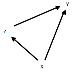
3.5 Unshielded Colliders and Asymmetry
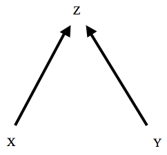
Suppose that X and Y are both direct causes of Z, and that neither X nor Y is a direct cause of the other. The relevant sub-graph is shown above in Figure 6. In such a case, the variable Z is said to be an unshielded collider. The (CMC) entails that X and Y will be independent conditional upon their parents, but it does not entail that they will be independent conditional upon any set containing Z. If the graph is faithful to the distribution, then X and Y will be probabilistically dependent conditional upon any set containing Z. For example, suppose that Figure 6 is the complete graph, and that the probability distribution satisfies both the MC and the Faithfulness Condition. Then X and Y will be probabilistically independent, but probabilistically dependent conditional upon Z. This is exactly the opposite of what we find in a common cause structure: if Z is a common cause of X and Y, then X and Y will be probabilistically dependent, but independent conditional upon Z. Many people find it counterintuitive that the probabilistically independent X and Y become dependent when we condition upon Z. This is related to Berkson' Paradox in probability, and is the source of well-known Monte Hall paradox.
Despite Reichenbach's focus on common cause structures, unshielded colliders actually prove to be more useful for inferring causal structure from probabilities. The reason for this is that the screening-off relation that holds when Z is a common cause of X and Y also holds when Z is a causal intermediate between X and Y. By contrast, the opposite probabilistic relationship is unique to unshielded colliders. Many of the algorithms that have been developed for inferring causal structure from probabilities work by searching for unshielded colliders. See, e.g. SGS (2000, Chapter 5).
The different probabilistic behavior of common causes and unshielded colliders seems to partially fulfill Reichenbach's hope of providing a probabilistic criterion for the direction of causation. When we have multiple causal arrows that are either all pointing inward toward a variable Z, or outward away from it, we are often able to infer from the probabilistic dependence relations which way they are pointing.
Further Reading: Hausman (1998), Chapters 10–12; Spirtes, Glymour and Scheines (2000), Chapters 1, 3, and 5.
3.6 Intervention
A conditional probability such as P(Y = y | X = x) gives us the probability that Y will take the value y, given that X has been observed to take the value x. Often, however, we are interested in predicting the value of Y that will result if we intervene to set the value of X equal to some particular value x. Pearl writes P(Y = y | do(X = x)) to characterize this probability. What is the difference between observation and intervention? When we merely observe the value that a variable takes, we are learning about the value of the variable when it is caused in the normal way, as represented in our causal model. Information about the value of the variable will also provide us with information about its causes, and about other effects of those causes. However, when we intervene, we override the normal causal structure, forcing a variable to take a value it might not have taken if the system were left alone. In the ideal case, the value of the variable is determined completely by our intervention, the causal influence of the other variables being completely overridden. Graphically, we can represent the effect of this intervention by eliminating the arrows directed into the variables intervened upon. Such an intervention is sometimes described as ‘breaking’ those arrows. See Woodward (2003) and the entry for Causation and Manipulation for a more detailed characterization of such interventions.
A causal model can be used to predict the effects of such an intervention. Indeed, this is what gives the model its distinctively causal interpretation. Otherwise, we might view the graph G as merely being an economical encoding of probabilistic dependence relations (which is how Pearl conceived it in his earlier book, Pearl (1988).) As Pearl (2000) conceives of it, quantities such as P(Y = y | do(X = x)), or more generally P(Y = y | X =x, do(Z = z)), are distinctively causal, and the central task of probabilistic causation is the identification of such causal quantities with probabilistic expressions that are free of the ‘do’ operator.
Suppose we have a causal model in which the probability distribution P satisfies the MC on the graph G over the variable set V = {X1, X2, …, Xn}. Recall that P will factorize as follows:
P(X1, X2, …, Xn) = Πi P(Xi | PA(Xi))
Now suppose we intervene by setting the value of Xk to xk, without disturbing the causal relationships among any of the other variables. The post-intervention probability P′ is the result of altering the factorization as follows:
P′(X1, X2, …, Xn) = P′(Xk) × Πi≠k P(Xi | PA(Xi)),
where P′(Xk = xk) = 1. The conditional probabilities of the form P(Xi | PA(Xi)) for i ≠k remain unchanged by the intervention.
Both SGS (2000) and Pearl (2000) generalize this result in a number of ways. SGS prove a theorem, theorem 3.6 of SGS (2000), which they dub the ‘manipulation theorem’, that generalizes this formula to cover a much broader class of interventions
Pearl develops an axiomatic system he calls the ‘do-calculus’ to determine the effects of interventions. This calculus consists of three axioms that allow for the substitution of probability formulae involving the ‘do’ operator. This calculus does not require that the probability distribution satisfy the MC (nor Faithfulness), and so it may be applied to variable sets even when there are unobserved common causes. Huang and Valtorta (2006) and Shpitser and Pearl (2006) have independently proven this calculus to be complete, so that it characterizes all of the post-intervention probabilities that can be expressed in terms of simple conditional probabilities. Typically, this requires considerably less specific causal knowledge than the construction of ‘background contexts’ discussed in Section 2.5 above. Zhang (2007) provides a weaker version of the do-calculus that does not require knowledge of the causal structure (i.e., where only causal structure that can be reliably inferred from the original probabilities is used).
Further Reading: Spirtes, Glymour and Scheines (2000), chapter 3, Pearl (2000), chapter 3.
3.7 Statistical Distinguishability and Reduction
The original hope of Reichenbach and Suppes was to provide a reduction of causation to probabilities. To what extent has this hope been realized within the causal modeling framework? Causal modeling does not offer a reduction in the traditional philosophical sense; that is, it does not offer an analysis of the form ‘X causes Y if and only if…’ where the right hand side of the bi-conditional makes no reference to causation. Instead, it offers a series of postulates about how causal structure constrains the values of probabilities. Still, if we have a set of variables V and a probability distribution P on V, we may ask if P suffices to pick out a unique causal graph G on V. More generally, if G and G′ are distinct causal graphs on V, when is it possible to eliminate one or the other using the probability distribution over V? When there are probability distributions that are compatible with one, but not the other, we will say that the graphs are statistically distinguishable. There are a variety of notions of statistical distinguishability. There may be some probability measure that is compatible with G but not G′, or vice versa; or it may be that all measures compatible with G are incompatible with G′. Moreover, it may depend upon which conditions we impose on the relationship between the graph and the probability distribution; for example, whether we require only the (CMC), or also the Minimality or Faithfulness Conditions.
It will not always be possible to distinguish causal graphs. For example, consider a set V containing the three variables X, Y, and Z. The three structures where (i) X causes Y, which causes Z; (ii) Z causes Y, which causes X; and (iii) Y is a common cause of X and Z are statistically indistinguishable on the basis of conditional independence relations, even if we assume both the (CMC) and the faithfulness condition. All three imply that Y screens X off from Z, and that there are no further non-trivial relations of conditional or unconditional independence. On the other hand, the structure where X and Z are both causes of Y is statistically distinguishable from all other structures if we assume the (CMC) and Faithfulness Conditions. This model implies that X and Z are unconditionally independent, and that there are no further non-trivial conditional or unconditional independence relations. No other graph on the three variables implies just these dependence relations.
There a number of important results establishing that it is possible to determine causal structure from probabilities in certain special cases. Three such results are described in the supplementary document:
Three Results Concerning Statistical Distinguishability
Further Reading: Pearl (2000), Chapter 1; Spirtes, Glymour and Scheines (2000), Chapter 4.
4. Other Theories
A number of authors have advanced probabilistic theories of causation that don't fit neatly under any of the headings in Sections 2 and 3. Some of these are probabilistic extensions of other theories of causation, such as counterfactual theories or manipulability theories.
4.1 Counterfactual Theories
A leading approach to the study of causation has been to analyze causation in terms of counterfactual conditionals. A counterfactual conditional is a subjunctive conditional sentence, whose antecedent is contrary-to-fact. Here is an example: “if Mary had not smoked, she would not have developed lung cancer.” In the case of indeterministic outcomes, it may be appropriate to use probabilistic consequents: “if Mary had not smoked, her probability of developing lung cancer would have been only .02.” A number of attempts have been developed to analyze causation in terms of such probabilistic counterfactuals. Since these counterfactuals refer to particular events at particular times, counterfactual theories of causation are theories of singular causation.
David Lewis is the best-known advocate of a counterfactual theory of causation. In Lewis (1986b), he presented a probabilistic extension to his original counterfactual theory of causation (Lewis 1973). According to Lewis's theory, the event E is said to causally depend upon the distinct event C just in case both occur and the probability that E would occur, at the time of C′s occurrence, was much higher than it would have been at the corresponding time if C had not occurred. This counterfactual is to be understood in terms of possible worlds: it is true if, and only if, in the nearest possible world(s) where C does not occur, the probability of E is much lower than it was in the actual world. On this account, the relevant notion of ‘probability-raising’ is not understood in terms of conditional probabilities, but in terms of unconditional probabilities in different possible worlds. Causal dependence is sufficient but not necessary for causation. Causation is defined to be the ancestral of causal dependence; that is:
(Lewis) C causes E just in case there is a sequence of events D1, D2, …, Dn, such that D1 causally depends upon C, D2 causally depends upon D1, …, E causally depends upon Dn.
This definition guarantees that causation will be transitive: if C causes D, and D causes E, then C causes E. This modification is also useful in addressing certain types of preemption. Nonetheless, it has been widely acknowledged that Lewis's theory has problems with other types of preemption, and with probability-raising non-causes (see Section 2.10 above).
There have been a number of attempts to revise Lewis's counterfactual probabilistic theory of causation so as to avoid these problems. In the final postscript of Lewis (1986b), Lewis proposed a theory in terms of ‘quasi-dependence’ that could naturally be extended to the probabilistic case. Lewis (2000) presents a new counterfactual theory of deterministic causation, in which he concedes that there are problems in probabilistic causation that his account is not yet able to handle. Peter Menzies (1989) offers a revision of Lewis's original theory that pays attention to the continuous processes linking causes and effects. This account is designed to handle cases of probability-raising non-causes. Menzies (1996) concedes that this account still has problems with certain types of preemption, and abandons it in favor of the theory discussed in Section 4.2 below. Paul Noordhof (1999) develops an elaborite counterfactual probabilistic theory of causation designed to deal with preemption, and additional problems relating to causes that affect the time at which an event occurs. Ramachandran (2000) presents some apparent counterexamples to this theory, to which Noordhof (2000) responds. Schaffer (2001) offers an account according to which causes raise the probability of specific processes, rather than individual events. This account is also motivated by the problems of preemption and probability-lowering causes.
Further Reading: Lewis (1973, 1986b); Menzies (1989, 2009), Noordhof (1999), Paul (2009). See the entry on ‘Causation: Counterfactual Theories’ for extensive discussion of some of the issues presented here, in particular, problems relating to preemption.
4.2 The Canberra Plan
“The Canberra Plan” refers to a strategy for analyzing theoretical terms advocated by David Lewis (1972), and named for its popularity among philosophers affiliated with the Australian National University. The strategy involves first articulating the ‘folk theory’ of a concept, which is done by enumerating a series of ‘platitudes’ about the concept. This folk theory, however, is not the final story on the concept. Indeed, it is typically recognized that the platitudes will admit of counterexamples. Instead, the term is taken to refer to that natural entity, property or relation that comes closest to satisfying the folk theory.
Menzies (1996) applied this strategy to the concept of causation. Menzies enumerated three platitudes:
- Causation is a relation that holds between distinct events.
- Causation is an intrinsic relation. That is, if C causes E, this relation holds in virtue of the intrinsic properties of C and E and of other events in their immediate spatiotemporal vicinity.
- C causes E when C raises the probability of E (as characterized by probabilistic counterfactuals of the sort discussed in Section 4.1).
Menzies notes that 3 is known to have counterexamples, such as those described in Section 2.10 above. Nonetheless, 3 is typically true. Causation, then, is the intrinsic relation that typically holds between distinct events when one raises the probability of the other. It is an empirical question just what this relation is. Menzies (1996) does not offer a definitive answer, but conjectures that it might be the transfer of energy or momentum. This identification, however, would seem to rule out many cases of prevention and causation by omission, as argued forcefully by Schaffer (2000).
Further Reading: Menzies (1996). See Dowe (2009) and the entry on Causal Processes for discussion of some of the issues involved in identifying causation with the transfer of energy or momentum.
4.3 Interventionist Theories
Woodward (2003) offers an account of causation according to which a causal relationship is a difference-making relationship between variables that is stable under interventions. To say that the relationship is difference-making is to say that the value taken by one variable makes a difference to the value taken by another. This relationship can be deterministic, as when the increase in the charge on a plate causes a corresponding increase in the acceleration of a test particle; but it can also be probabilistic, as when an increase in the amount that an individual smokes increases her probability of lung cancer.
An intervention on the variable X with respect to the variable Y is a change in the value of some variable I that is a cause of X but must also meet a number of further conditions; for example, I must not have a path-specific effect on Y via any path that does not go through X. For example, consider the common cause structure shown in Figure 1 above. Although we could, in principle, affect the reading of a barometer by changing the atmospheric pressure, this would not count as an intervention on the barometer reading with respect to the occurrence of a storm. While the barometer reading is correlated with the weather, this correlation would disappear if the barometer reading were brought about by an intervention (for example, if we were to put the barometer in the refrigerator). The genuinely causal correlations are the ones that would persist under this sort of intervention.
Further Reading: Woodward (2003, 2009). See the entry on ‘Causation and Manipulability’ for extensive discussion.
4.4 Singular Causation and the Evolution of Probabilities in Time
Ellery Eells (1991, Chapter 6), and Igal Kvart (2004) have developed probabilistic theories of singular causation that depend upon the way in which probabilities change over time. These theories are presented in the supplementary document:
Singular Causation and the Evolution of Probabilities in Time
Bibliography
- Arntzenius, Frank, (1990). “Physics and Common Causes”, Synthese, 82: 77–96.
- Beebee, Helen, Christopher Hitchcock, and Peter Menzies (eds.), (2009). The Oxford Handbook of Causation, Oxford: Oxford University Press.
- Bennett, Jonathan, (1988). Events and Their Names, Indianapolis and Cambridge: Hackett.
- Billingsley, Patrick, (1995). Probability and Measure, Third Edition. New York: Wiley.
- Carroll, John, (1991). “Property-level Causation?” Philosophical Studies, 63: 245–70.
- Cartwright, Nancy, (1979). “Causal Laws and Effective Strategies,” Noûs, 13: 419–437.
- –––, (1989). Nature's Capacities and Their Measurement, Oxford: Oxford University Press.
- –––, (1993). “Marks and Probabilities: Two Ways to Find Causal Structure,” in Fritz Stadler (ed.), Scientific Philosophy: Origins and Development, Dordrecht: Kluwer.
- –––, (2007). Hunting Causes and Using Them, Cambridge: Cambridge University Press.
- Collins, John, Ned Hall, and L.A. Paul (eds.), (2004). Causation and Counterfactuals, Cambridge MA: MIT Press.
- Davis, Wayne, (1988). “Probabilistic Theories of Causation,” in James Fetzer (ed.), Probability and Causality, Dordrecht: Reidel, pp. 133–160.
- Dowe, Phil, (2000). Physical Causality, Cambridge: Cambridge University Press.
- –––, (2004). “Chance-lowering Causes,” in Dowe and Noordhof (2004), pp. 28–38.
- –––, (2009). “Causal Process Theories,” in Beebee, Hitchcock, and Menzies (2009), pp. 213 - 233.
- –––, and Noordhof, Paul (eds.), (2004). Cause and Chance, London and New York: Routledge.
- Dupré, John, (1984). “Probabilistic Causality Emancipated,” in Peter French, Theodore Uehling, Jr., and Howard Wettstein, eds., (1984) Midwest Studies in Philosophy IX, Minneapolis: University of Minnesota Press, pp. 169–175.
- Eells, Ellery, (1991). Probabilistic Causality, Cambridge, U.K.: Cambridge University Press.
- Ehring, Douglas, (2009). “Causal Relata,” in Beebee, Hitchcock, and Menzies (2009), pp. 387–413.
- Feller, William, (1968). An Introduction to Probability Theory and its Applications, New York: Wiley.
- Galavotti, Maria Carla, (2005). Philosophical Introduction to Probability, Stanford: CSLI Publications.
- Geiger, Daniel, (1987). “Towards the Formalization of Informational Dependencies,” Technical Report 880053 (R-102), Los Angeles: UCLA Cognitive Systems Laboratory.
- Gillies, Donald, (2000). Philosophical Theories of Probability, London and New York: Routledge.
- Glymour, Clark, (2009). “Causality and Statistics,” in Beebee, Hitchcock, and Menzies (2009), pp. 498–522.
- ––– and Gregory Cooper, (1999). Computation, Causation, and Discovery, Cambridge, MA: MIT Press.
- Good, I. J., (1961). “A Causal Calculus I,” British Journal for the Philosophy of Science, 11: 305–18.
- –––, (1962). “A Causal Calculus II,” British Journal for the Philosophy of Science, 12: 43–51.
- Hausman, Daniel, (1998). Causal Asymmetries, Cambridge: Cambridge University Press.
- –––, (1999). “The Mathematical Theory of Causation,” British Journal for the Philosophy of Science, 50: 151–62.
- Hausman, Daniel, and Woodward, James, (1999). “Independence, Invariance, and the Causal Markov Condition,” British Journal for the Philosophy of Science, 50: 1–63.
- –––, (2004). “Modularity and the Causal Markov Condition: a Restatement,” British Journal for the Philosophy of Science, 55: 147–61.
- Hempel, Carl G., (1965). “Aspects of Scientific Explanation,” in Aspects of Explanation and Other Essays, New York: Free Press, pp. 331–496.
- Hesslow, Germund, (1976). “Discussion: Two Notes on the Probabilistic Approach to Causality,” Philosophy of Science, 43: 290–292.
- Hitchcock, Christopher, (1995). “The Mishap at Reichenbach Fall: Singular vs. General Causation,” Philosophical Studies, 78: 257–291.
- –––, (1996). “Farewell to Binary Causation,” Canadian Journal of Philosophy, 26: 267–282.
- –––, (2001). “A Tale of Two Effects,” Philosophical Review, 110: 361–396.
- –––, (2004a). “Do All and Only Causes Raise the Probabilities of Effects?” in Collins, Hall and Paul (2004), pp. 403–418.
- –––, (2004b). “Routes, Processes, and Chance Lowering Causes,” in Dowe and Noordhof (2004), pp. 138–151.
- –––, (2009). “Causal Models,” in Beebee, Hitchcock, and Menzies (2009), pp. 299–314.
- Horwich, Paul, (1987). Asymmetries in Time, Cambridge, MA: MIT Press.
- Huang, Yimin and Marco Valtorta, (2006). “Pearl's Calculus of Intervention Is Complete,” Proceedings of 22nd Annual Conference on Uncertainty in Artificial Intelligence, Arlington, VA: AUAI Press.
- Hume, David, (1748). An Enquiry Concerning Human Understanding.
- Humphreys, Paul, (1989). The Chances of Explanation: Causal Explanations in the Social, Medical, and Physical Sciences, Princeton: Princeton University Press.
- Kvart, Igal, (2004). “Causation: Probabilistic and Counterfactual Analyses,” in Collins, Hall and Paul (2004), pp. 359–387.
- Kyburg, Henry, (1965). “Discussion: Salmon's Paper”, Philosophy of Science, 32: 147–151.
- Lewis, David, (1972). “Psychophysical and Theoretical Identifications,” Australasian Journal of Philosophy 50: 249–58.
- –––, (1973). “Causation,” Journal of Philosophy, 70: 556–567.
- –––, (1986a). “Events,” in Lewis (1986c), pp. 241–270.
- –––, (1986b). “Postscripts to ‘Causation’,” in Lewis (1986c), pp. 173–213.
- –––, (1986c). Philosophical Papers, Volume II, Oxford: Oxford University Press.
- –––, (2000). “Causation as Influence,” Journal of Philosophy, 97: 182–197.
- Mellor, Hugh, (2004). “For Facts as Causes and Effects,” in Collins, Hall and Paul (2004), pp. 309–324.
- Menzies, Peter, (1989). “Probabilistic Causation and Causal Processes: A Critique of Lewis,” Philosophy of Science, 56: 642–63.
- –––, (1996). “Probabilistic Causation and the Pre-emptionProblem”, Mind, 105: 85–117.
- –––, (2009). “Platitudes and Counterexamples,” in Beebee, Hitchcock, and Menzies (2009), pp. 341–367.
- Neapolitan, Richard, (2004). Learning Bayesian Networks, Upper Saddle River, NJ: Prentice Hall.
- Noordhof, Paul, (1999). “Probabilistic Causation, Preemption and Counterfactuals,” Mind, 108: 95–125.
- –––, (2000). “Ramachandran's Four Counterexamples,” Mind, 109: 315–324.
- Paul, L.A., (2009). “Counterfactual Theories of Causation,” in Beebee, Hitchcock, and Menzies (2009), pp. 158–184.
- Pearl, Judea, (1988). Probabilistic Reasoning in Intelligent Systems, San Francisco: Morgan Kaufman.
- –––, (1995). “Causal Diagrams for Empirical Research,” Biometrika, 82: 669–710.
- –––, (2000). Causality: Models, Reasoning, and Inference, Cambridge: Cambridge University Press.
- –––, (2001). “Direct and Indirect Effects,” Proceedings of the Seventeenth Conference on Uncertainty in Artificial Intelligence, San Francisco, CA: Morgan Kaufmann, pp. 411–420
- Pearl, Judea, and Verma, Thomas, (1991). “A Theory of Inferred Causation,” Principles of Knowledge Representation and Reasoning: Proceedings of the 2nd International Conference, San Mateo, CA: Morgan Kaufman, pp. 441–52.
- Price, Huw, and Brad Weslake, (2009). “Causation and Time,” in Beebee, Hitchcock, and Menzies (2009), pp. 414–446.
- Psillos, Stathis, (2009). “Regularity Theories of Causation,” in Beebee, Hitchcock, and Menzies (2009), pp. 131–157.
- Ramachandran, Murali, (2000). “Noordhof on Probabilistic Causation,” Mind, 109: 309–313.
- Reichenbach, Hans, (1925). “Die Kausalstruktur der Welt und der Unterschied von Vergangenheit und Zukunft,” Sitzungsberichte der Bayerische Akademie der Wissenschaft, November: 133–175. English translation ‘The Causal Structure of the World and the Difference between Past and Future’, in Maria Reichenbach and Robert S. Cohen (eds.), Selected Writings: 1909–1953, Vol. II (Dordrecht and Boston: Reidel), pp. 81–119.
- –––, (1956). The Direction of Time, Berkeley and Los Angeles: University of California Press.
- Salmon, Wesley, (1971). “Statistical Explanation,” in Statistical Explanation and Statistical Relevance, ed. W. Salmon, Pittsburgh: University of Pittsburgh Press, pp. 29–87.
- –––, (1980). “Probabilistic Causality,” Pacific Philosophical Quarterly, 61: 50–74.
- –––, (1984). Scientific Explanation and the Causal Structure of the World, Princeton: Princeton University Press.
- Schaffer, Jonathan, (2000). “Causation by Disconnection,” Philosophy of Science, 67: 285–300.
- –––, (2001). “Causes as Probability-Raisers of Processes,” Journal of Philosophy, 98: 75–92
- –––, (2005). “Contrastive Causation,” Philosophical Review, 114: 327–358.
- Scheines, Richard, (1997). “An Introduction to Causal Inference” in V. McKim and S. Turner (eds.), Causality in Crisis? (Notre Dame: University of Notre Dame Press), pp. 185–199.
- Shannon, Claude, (1948). “A Mathematical Theory of Communication,” Bell System Technical Journal, 27: 379–423, 623–56.
- Shimizu, Shohei, Patrick Hoyer, Aapo Hyvärinen, and Antti Kermine, (2006). “A Linear Non-Gaussian Acyclic Model for Causal Discovery,” Journal of Machine Learning Research, 7: 2003–2030.
- Shpister, Ilya and Judea Pearl, (2006). “Identification of Conditional Interventional Distributions,” in R. Dechter and T.S. Richardson (eds.), Proceedings of the Twenty-Second Conference on Uncertainty in Artificial Intelligence, Corvallis, OR: AUAI Press, pp. 437–444.
- Skyrms, Brian, (1980). Causal Necessity, New Haven and London: Yale University Press.
- Sloman, Steven, (2005). Causal Models, Oxford: Oxford University Press.
- Sober, Elliott, (1985). “Two Concepts of Cause,” in Peter Asquith and Philip Kitcher (eds.), PSA 1984, Vol. II (East Lansing: Philosophy of Science Association), pp. 405–424.
- –––, (2001). “Venetian Sea Levels, British Bread Prices, and the Principle of the Common Cause,” British Journal for the Philosophy of Science, 52 (2): 3311–346.
- Spirtes, Peter, Clark Glymour, and Richard Scheines, (2000). Causation, Prediction and Search, second edition, Cambridge, MA: M.I.T. Press.
- Spirtes, Peter, and Richard Scheines, (2004). “Causal Inference of Ambiguous Manipulation,” Philosophy of Science, 71 (Supplement): S833–S845.
- Suppes, Patrick, (1970). A Probabilistic Theory of Causality, Amsterdam: North-Holland Publishing Company.
- Twardy, Charles, and Kevin Korb, (2004). “A Criterion of Probabilistic Causation,” Philosophy of Science, 71: 241–262.
- Verma, Thomas, and Judea Pearl, (1988). “Causal Networks: Semantics and Expressiveness,” Proceedings of the 4th Workshop on Uncertainty in Artificial Intelligence, Minneapolis, MN and Mountain View, CA, pp. 352–359.
- Williamson, Jon, (Forthcoming). “Probabilistic Theories of Causation,” in Beebee, Hitchcock, and Menzies (Forthcoming).
- Woodward, James, (1990). “Supervenience and Singular Causal Claims,” in Dudley Knowles, ed., Explanation and its Limits, Cambridge, U.K: Cambridge University Press, pp. 211–246.
- –––, (2003). Making Things Happen: A Theory of Causal Explanation, Oxford: Oxford University Press.
- –––, (2009). “Agency and Intervention Theories of Causation,” in Beebee, Hitchcock, and Menzies (2009), pp. 234–264.
- Zhang, Jiji, (2007). “Generalized Do-Calculus with Testable Causal Assumptions,” Proceedings of the 11th International Conference on Artificial Intelligence and Statistics. [Available online]
Other Internet Resources
- Causal Analysis and Theory in Practice
- Causality, webpage on Judea Pearl's book.
- The Tetrad Project
- The Carnegie Mellon Curriculum on Causal and Statistical Reasoning
Related Entries
causation: and manipulability | causation: backward | causation: causal processes | causation: counterfactual theories of | causation: in the law | causation: the metaphysics of | conditionals: counterfactual | decision theory: causal | determinism: causal | events | facts | Hume, David | Kant, Immanuel: and Hume on causality | Mill, John Stuart | physics: Reichenbach's common cause principle | probability, interpretations of | properties | quantum mechanics | quantum mechanics: action at a distance in | quantum theory: the Einstein-Podolsky-Rosen argument in | Reichenbach, Hans | scientific explanation | Simpson's paradox | time
Acknowledgments
Thanks to Clark Glymour, Judea Pearl, Richard Scheines, Elliott Sober, and Jim Woodward for detailed comments, corrections, and discussion.