This is a file in the archives of the Stanford Encyclopedia of Philosophy.

Conservation Biology

Conservation biology emerged as an organized academic discipline in the United States in the 1980s though much of its theoretical framework was originally developed in Australia. Significant differences of approach in the two traditions were resolved in the late 1990s through the formulation of a consensus framework for the design and adaptive management of conservation area networks. This entry presents an outline of that framework along with a critical analysis of conceptual issues concerning the four theoretical problems that emerge from it: (i) place prioritization for conservation action; (ii) the selection of surrogates for biodiversity in conservation planning; (iii) the assessment of vulnerability of conservation areas; and (iv) the synchronization of incommensurable criteria including socio-economic constraints on conservation planning.

• 1. Introduction and Historical Background
• 2. The Consensus Framework
• 3. Place Prioritization
• 4. Surrogacy
• 5. Vulnerability and Viability
• 6. Multiple Criterion Synchronization
• 7. Final Remarks
• Bibliography
• Other Internet Resources
• Related Entries

---

1. Introduction and Historical Background

Conservation biology only emerged as a distinct professional enterprise with its own practices, cultures, and social institutions in the 1980s. In one sense, it is possible not only to place and date, but even to time, its emergence as an organized discipline: at about 5 p.m. (EST), 8 May 1985, in Ann Arbor, Michigan, at the end of the Second Conference on Conservation Biology.^[1] Two ad hoc committees, chaired by Jared Diamond and Peter Brussard, had met during the conference to discuss the need for a new society and a new journal. Following their recommendations, an informal motion to found the society was passed, and Michael E. Soulé was given the task of organizing the new society. It was decided to found a new journal, Conservation Biology. That a successful European journal, Biological Conservation, devoted to the same topic, had been in existence since 1968 apparently went unnoticed. Participants at the Ann Arbor conference seem to have been convinced that they were boldly going where no one had gone before.

In another sense, a science of biological conservation is centuries old, going back to the traditions of forest and game management developed in many countries, particularly Germany and India, in the eighteenth and nineteenth centuries. There is as yet no systematic historical or philosophical analysis of the question whether modern conservation biology should be viewed as an enterprise distinct from these earlier disciplines rather than as a development from them. There are also interesting questions about the relation of conservation biology to more traditional biological sub-disciplines, especially ecology. This entry will return to those questions after recounting the historical context of the emergence of conservation biology and explicating its current conceptual structure.

Returning to Ann Arbor, with hindsight, it is hard not to attribute the sense of self-laudatory pioneering mission among the participants of that conference to little more than a strange but persistent myopia in the vision of the conservation community of the United States during that period. Two factors contributed to that myopia: (i) a genuine lack of awareness of developments elsewhere, particularly in Australia (see below), that were critically shaping the conceptual structure and practices of the emerging discipline; and (ii) the Ann Arbor conference constituted a sharp break from an immediate past during which some highly uncritical attempts to apply ecological principles to problems of biological conservation had resulted in publicly recognized failures (see below). Participants at the Ann Arbor meeting clearly hoped that the development of an explicit agenda for a new discipline represented a transition to maturity that would prevent — or at least discourage — such mistakes in the future.

In north America, particularly in the United States, ecologists had generally begun to be concerned with biological conservation only in the 1960s when large-scale anthropogenic conversion of neotropical habitats had forced them to recognize the possibility that their field research sites might soon disappear. One result of such habitat conversion was that species were being driven to extinction before they were scientifically described and studied. Given the well-established north American tradition of designating national parks for nature conservation, a not unexpected response to this problem of habitat destruction was to pursue the creation of nature reserve networks throughout the world. The problem of reserve network design became the first theoretical problem that conservation biology could uniquely claim at its own. In the United States in the 1970s ecologists tried to solve this problem by applying island biogeography theory^[2] on the assumption that reserves are adequately modeled as viable islands in oceans of anthropogenically transformed habitat (May 1975, Diamond & May 1976). Within ecology, despite its early promise, island biogeography theory was coming under increasing critical experimental scrutiny during this period (Simberloff 1976). Nevertheless, its principles were adopted in the context of reserve network design even by some international conservation agencies^[3] without any attempt to assess whether its empirical basis was sound. The attempt to use island biogeography for reserve network design soon generated a major controversy, whether single large or several small (SLOSS) reserves were preferable.^[4] Though this controversy persisted for almost a decade, its ultimate resolution was that it had no solution: by 1985 it was clear that the answer depended on highly contingent local factors (Soulé & Simberloff 1986). The Ann Arbor conference occurred in this context in which it had become clear that conservation biology needed new foundations if it was ever to develop as a successful discipline.

For attempts to use island biogeography theory in reserve network design the most telling criticism came from Margules, Higgs and Rafe (1982) who pointed out both that the model had not been empirically established and that there were important disanalogies between biological reserves and islands. In particular, areas between reserves were not as inhospitable to species in the reserves as oceans were to insular species. Graeme Caughley, Chris Margules, Mike Austin, Bob Pressey, and several others, mainly in Australia, pioneered a radically different approach to biological conservation than what was emerging in north America. This approach partly reflects a unique Australian experience including the fact that extensive habitat conversion had only begun relatively recently, leaving much greater scope for systematic biodiversity conservation compared to Asia, Europe, or even North America (Margules 1989). More importantly it reflects the practical background of most Australian conservation biologists in the management of wildlife and other biological resources (rather than in academic research). This resulted in an explicitly pragmatic attitude to the solution of biodiversity conservation problems. The role of academic ecology was comparatively limited. Rather, the version of conservation biology developed by the Australian school relied on generic “common sense” ecological heuristics which will be emphasized in the discussion below. There was also little explicit consideration of the ethical or normative basis of conservation practice, again in sharp contrast to practice in the United States^[5] even though, by paying explicit attention to socio-political factors, this approach was implicitly incorporates anthropocentric norms at every stage. A 1989 volume of Biological Conservation edited by Margules brought the Australian approach to biological conservation to a broader audience.^[6] The Australians were also the first to propose a reasonable solution to the problem of reserve network design (see below).^[7]

In the United States, things moved quickly from the Ann Arbor conference. In December 1985, Soulé published a long manifesto, “What is Conservation Biology?” in BioScience, the journal most visible to the academic and, especially, the non-academic biological community in the United States. Soulé proclaimed that a new inter-disciplinary science, conservation biology, based on both substantive and normative ethical foundations, had been recently created to conserve what still remained of Earth's biological heritage (Soulé 1985). This science was ultimately prescriptive: it prescribed management plans for the conservation of biological diversity at every level of organization. Setting the tone for much of the discussion during the early years of North American conservation biology, Soulé emphasized that the new field was a “crisis discipline.” The first issue of Conservation Biology appeared in May 1987, and the first annual meeting of the new society was held in Montana State University in June 1987. Within ecology, in 1986, Daniel Janzen published an influential exhortation, “The Future of Tropical Ecology,” urging ecologists to undertake the political activism necessary for conservation: “If biologists want a tropics in which to biologize [sic], they are going to have to buy it with care, energy, effort, strategy, tactics, time, and cash. I cannot overemphasize the urgency as well as the responsibility… If our generation does not do it, it won't be there for the next. Feel uneasy? You had better. There are no bad guys in the next village. They is us [sic]” (Janzen 1986, 306).

Thus, between 1985 and 1987, conservation biology emerged in the United States as an organized academic discipline. Its focus became “biodiversity,” a term that entered the everyday and scientific lexicons around 1988. This neologism was coined by Walter G. Rosen at some point during the organization of the 21 –24 September 1986 “National Forum on BioDiversity” held in Washington, D. C., under the auspices of the US National Academy of Sciences and the Smithsonian Institution.^[8] The new term was initially intended as nothing more than a shorthand for “biological diversity” for use in internal paperwork during the organization of that forum. However, from its very birth it showed considerable promise of transcending its humble origins. By the time the proceedings of the forum were published, Rosen's neologism — though temporarily mutated as “BioDiversity” (Wilson 1988) — had eliminated all rivals to emerge as the title of the book that emerged from that conference.

The term “biodiversity” found immediate wide use following its introduction.^[9] The first journal with “biodiversity” in its title, Canadian Biodiversity, appeared in 1991, changing its name to Global Biodiversity in 1993; a second, Tropical Biodiversity, began appearing in 1992; Biodiversity Letters and Global Biodiversity followed in 1993. A sociologically synergistic interaction between the use of the term “biodiversity” and the growth of conservation biology as a discipline led to a re-configuration of environmental studies in which biodiversity conservation became a central focus of environmental concern. However, for all its appeal, “biodiversity” has proved notoriously difficult to define — see the entry on biodiversity. In 1989, Soulé and Kohm published a primer on research priorities for the field. It was catholic in scope, including demography, ecology, genetics, island biogeography, public policy, and systematics, as components of conservation biology. It called for massive biological surveys, especially in the neotropics, and for the circumvention of legal barriers to the use of US federal funds for the purchase of land in other countries (Soulé & Kohm 1989). In 1993, Primack produced the first textbook of conservation biology, and in 1994, Meffe and Carroll followed with a more comprehensive effort.^[10]

In the United States, the legislative context of the 1970s largely determined the course of research in conservation biology in its early years, an exemplary case of the social determination of science.^[11] The decisive event was the passage of the Endangered Species Act (ESA) in 1973 at the end of a long history of US federal conservationist legislation including the Endangered Species Preservation and Conservation Acts (of 1966 and 1969, respectively) and the National Environmental Policy Act (1969). Subsequent amendments to the ESA required not only the listing of threatened and endangered species but also the designation of critical habitats and the design of population recovery plans. Equally important as the ESA was the 1976 National Forest Management Act (NFMA). This act required the Forest Service to “provide for diversity of plant and animal communities based on the suitability and capability of the specific land area.”^[12] In 1979 the planning regulations developed to implement this provision required the Forest Service to “maintain viable populations of existing native and desired non-native vertebrate species in the planning area.”^[13]

Since populations of threatened and endangered species are generally small, attempts to implement this legislation naturally led to a focus on small populations subject to stochastic fluctuations in size, including extinction.^[14] In a 1978 dissertation, “Determining Minimum Viable Population Sizes: A Case Study of the Grizzly Bear,” influenced by the ESA, Mark L. Shaffer attempted to formulate a systematic framework for the analysis of effects of stochasticity on small populations. It introduced the concept of the minimum viable population (MVP), the definition of which involved several conventional choices that eventually came to be widely reified as definitive benchmarks: the probability of persistence that was deemed sufficient as a conservation goal, and the time up to which that probability had to be maintained were both matters of choice. One common choice was to define an MVP as a population that has a 95 % probability of surviving for the next 100 years^[15] both numbers are conventions with no firm biological basis though, for a definition to be of operational relevance in the field, some precise numbers such as these were necessary.^[16] The conservation and recovery plans for threatened and endangered species required under the ESA led almost inexorably to the risk assessment of small populations through stochastic analysis. The name population “vulnerability” analysis was used by Gilpin and Soulé in 1986; population “viability” analysis soon replaced it. The optimism of the late 1970s and early 1980s was reflected in Gilpin and Soulé's slogan: “MVP is the product, PVA the process” (Gilpin & Soulé 1986, 19).

However, by the late 1980s, it became clear that the concept of a MVP was at best of very limited use. Even for a single species, populations in slightly different habitat patches may show highly variable demographic trends, especially in the presence of stochasticity, resulting in high variability of estimated MVPs depending critically on local context.^[17] By the early 1990s PVA began to focus, instead, on estimating other only slightly more robust parameters such as the expected time to extinction. Had PVA been successful in providing empirically reliable estimates for such parameters, there would be no doubt about the centrality of its role in conservation planning. Indeed, it would justify Shaffer's rather grandiose 1994 claim: “Like physicists searching for a grand unified theory explaining how the four fundamental forces … interact to control the structure and fate of the universe, conservation biologists now seek their own grand unified theory explaining how habitat type, quality, quantity, and pattern interact to control the structures and fates of species. Population viability analysis (PVA) is the first expression of this quest.” (in Meffe & Carroll 1994, 305-306). Unfortunately, though over hundreds of PVAs have been performed, a common methodology for PVA, or a consensus about its value, is yet to emerge. Indeed, there is ample room for skepticism about the future of PVA in conservation biology (see Section 5, below).

In Australia, Margules and Caughley were among those who expressed such skepticism (Margules 1989; Caughley 1994). Caughley argued that two “paradigms”^[18] had emerged in conservation biology: a “small populations” paradigm and a “declining populations” paradigm. In PVA, the former dictated the use of stochastic models, the latter the use of deterministic models. Caughley argued that the former contributed little to the conservation of species in the wild because, beyond the trivial insight that small populations are subject to stochasticity, stochastic models do not provide insight into why species are at risk. Conservation has a better chance of success in the latter case since, with large populations, it is usually possible to design field experiments with appropriate controls to determine the ecological mechanisms of decline. Such experiments, in turn, should lead to new and badly needed theoretical explorations within the declining populations paradigm. Though Caughley did not couch his discussion in terms of national traditions, the small populations paradigm dominated research programs in the United States whereas the declining populations paradigm dominated the Australian tradition.

The period since 1995 has seen a new consensus framework for conservation biology emerging through the integration of insight from both traditions. In this framework, which will be the focus of Section 2, the central goal of conservation biology is the establishment of conservation area networks (CANs) and their adequate maintenance over time through appropriate management practices. From Australia, Margules and Pressey formulated this consensus framework in a 2000 article in Nature; in the United States, The Nature Conservancy presented a very similar framework in 2002, underscoring the extent of the consensus that has been achieved.^[19] Central to this consensus is the idea that conservation biology is about systematic conservation planning through what is sometimes called the “adaptive management”^[20] of landscapes. The actual framework that has been developed is one for the prioritization of places for biodiversity value^[21] and the formulation of management plans for the long-term (in principle, infinite) survival of the biological entities of interest. The entire process is supposed to be periodically iterated because species (or other units) may have become extinct — or have recovered from problems — in the interim, thereby changing the biodiversity value of a place, or because management practices may have turned out to be ineffective. This is the only sense in which the process is supposed to be adaptive. However, the framework is so new — it is yet to be fully implemented anywhere — that it is possible that this requirement of being adaptive will require changes in the framework as it is currently understood. At present “adaptive management” is only a slogan embodying a tantalizing promissory note.

2. The Consensus Framework

Table 2.1 details the consensus framework as a ten-stage process.^[22] The first stage is that of data collection. It is critical that the data be georeferenced. Almost all methods used in conservation planning assume that data are recorded in a Geographical Information System (GIS) model.^[23] It is at least arguable that the emergence of conservation biology as a science required the development of GIS technology and high-speed computation.^[24] At this stage, the biological entities that are of most conservation interest must be identified. Entities of conservation interest obviously include those that are at risk (for instance, those that are legally endangered or threatened in the United States.). However, they also include those that are endemic or rare, even if they are presently presumed not to be at risk, since their status can easily change with local transformations of habitat. Note that what biota are considered to be of conservation interest is typically not entirely determined by biology: charismatic species, including those of symbolic social value, such as national birds and animals, are often selected for attention irrespective of the intrinsic biological importance of their conservation. It is typical of conservation biology that purely scientific considerations are inextricably mixed with extraneous criteria when such decisions must be made.

The second stage of conservation planning consists of selecting surrogates to represent general biodiversity in the planning process. This aspect of conservation planning raises important conceptual issues — including the definition of biodiversity — and will be treated in detail in Section 4 . At the third stage, explicit targets and goals must be established for the conservation area network. Without explicit targets and goals, it would be impossible to assess the success (or failure) of a conservation plan. Once again, the choice of such targets and goals is not entirely determined biological considerations and provides ample scope for controversy. For instance, typically, two types of targets are used: (i) a level of representation for the expected coverage of each surrogate (that is, the expected or average number of occurrences of the surrgate) within a conservation area network (CAN); and (ii) these representation targets along with the maximum area of land that can be put under a conservation plan. A common target of type (i) is to set the level of representation at 10 % for the coverage of each surrogate.^[25] A common target of type (ii) is 10 % of the total area of a region.^[26] However, the actual numbers used are not determined — or even strongly suggested — by any biological criteria (that is, models or empirical data). Rather, they represent conventions arrived at by educated intuition: type (i) targets are supposed to reflect biological knowledge while type (ii) targets are usually a result of a “budget” of land that can be designated for conservation action. Soulé and Sanjayan (1998) have recently forcefully argued that these targets may lead to an unwarranted sense of security because their satisfaction can potentially be interpreted as suggesting that biodiversity is being adequately protected whereas the targets may only reflect socio-political constraints such as a limited budget. The issue remains controversial. As Section 3 will document, the methods for conservation planning that have so far been developed presume the existence of explicit targets. Other basically biological criteria — though not usually called targets — include the size, shape, dispersion, and connectivity of the conservation areas in a CAN. However, while it is generally accepted on ecological grounds that larger conservation areas are better than smaller ones, ecology does not specify how large is good enough. The questions of shape, dispersion, and connectivity, also remains controversial: while low dispersion or connectivity might help species migrate to find suitable habitat, etc., it can also lead to the spread of disease. Conservation biology is yet to address these issues adequately. The goals include socio-economic constraints which may also contribute to the biodiversity value of a conservation area by affecting its vulnerability.

At the fourth stage, the performance of existing conservation areas (if any) in satisfying the targets and other biological design criteria (established during the third stage) must be assessed. This assessment determines what conservation action (if any) should be taken. The fifth stage consists of prioritizing places for conservation action to satisfy the stated targets and goals of the third stage. This problem corresponds to the traditional problem of reserve network selection; it has been the central theoretical problem studied in conservation biology, and the one in which most progress has been made. It will be discussed in detail in Section 3. However, the current representation of biodiversity in a CAN does not ensure its persistence over time which also depends on the level of threat from ecological and anthropogenic factors. The sixth stage of systematic conservation planning consists of assessing such risks. This is often a difficult task, and much more remains uncertain than what is known. It will be discussed in Section 5. In the seventh stage, areas with poor prognosis for relevant biodiversity features are dropped and place prioritization is repeated.

Biodiversity conservation is not the only possible use of land. Competing uses, such as agriculture, recreation, or industrial development, place strong socio-economic and political constraints on environmental policy. The eighth stage consists of attempting to synchronize all these criteria. Once again interesting conceptual problems are encountered at this stage which will be treated in detail in Section 6. The end of the eighth stage produces a plan for implementation. An attempt at implementation constitutes the ninth stage of the systematic conservation planning process. If implementation is impossible, as it sometimes is because of the constraints encountered, new plans must be formulated. Such constraints include changing and limited budgets for designating areas for biodiversity conservation, economic costs connected with forgone opportunities, social costs, etc. This requires a return to the fifth stage. Finally, conservation action is not a one-time process. The status of biological entities changes over time. Consequently, the last stage consists of periodically repeating the entire process. This period of time between repetitions may be set in absolute terms (a specified number of years, once again chosen by convention) or determined by keeping track of explicitly specified indicators of the performance of a conservation area network.

Section 3 of this entry will discuss place prioritization (stages [5] and [7]). Though the choice of surrogates (stage [2]) occurs earlier in Table 2.1 than place prioritization, it will be discussed later, in Section 4, because it relies on the availability of place prioritization procedures. Section 5 will discuss vulnerability and viability (stage [6]). Section 6 will discuss multiple criterion synchronization (stage [7]). The other stages, which do not raise significant philosophically interesting issues, will not be discussed any further.^[27]

>Table 2.1
Systematic Conservation Action

1. Compile and assess biodiversity data for region: Compile available geographical distribution data on as many biotic and environmental parameters as possible at every level of organization; Collect relevant new data to the extent feasible within available time; remote sensing data should be easily accessible; systematic surveys at the level of species (or lower levels) will usually be impossible; Assess conservation status for biotic entities, for instance, their rarity, endemism, and endangerment; Assess the reliability of the data, formally and informally; in particular, critically analyze the process of data selection.

2. Identify biodiversity surrogates for region: Choose true surrogate sets for biodiversity for part of the region; be explicit about criteria used for this choice; Choose alternate estimator-surrogate sets that can be (i) quantified; and (ii) easily assessed in the field (using insights from Stage 1); Prioritize places using true surrogate sets; Prioritize places using as many combinations of estimator-surrogate sets as feasible; Assess which estimator-surrogate set is best on the basis of (i) efficiency and (ii) accuracy.

3. Establish conservation targets and goals: Set quantitative targets for surrogate coverage; Set quantitative targets for total network area; Set quantitative targets for minimum size for population, unit area, etc.; Set design criteria such as connectivity; Set precise goals for criteria other than biodiversity.

4. Review existing conservation areas: Estimate the extent to which conservation targets are met by the existing set of conservation areas.

5. Prioritize new places for potential conservation action Prioritize places for their biodiversity content to create a set of potential conservation area networks; Optionally, starting with the existing conservation area networks as a constraint, repeat the process of prioritization to compare results; Incorporate design criteria such as shape, size, dispersion, and connectivity.

6. Assess prognosis for biodiversity for each potential targeted place: Perform population viability analysis for as many species using as many models as feasible; Perform the best feasible habitat-based viability analysis to obtain a general assessment of the prognosis for all species in a potential conservation area; Assess vulnerability of a potential conservation area from external threats, using techniques such as risk analysis.

7. Refine networks of places targeted for conservation action: Delete the presence of surrogates from potential conservation areas if the viability of that surrogate is not sufficiently high; Run the prioritization program again to prioritize potential conservation areas by biodiversity value; Incorporate design criteria such as shape, size, dispersion, and connectivity.

8. Perform feasibility analysis using multiple criterion synchronization: Order each set of potential conservation areas by each of the criteria other than biodiversity; Find all best solutions; Discard all other solutions; Select one of the best solutions.

9. Implement conservation plan: Decide on most appropriate legal mode of protection for each targeted place; Decide on most appropriate mode of management for persistence of each targeted surrogate; If implementation is impossible return to Stage 5; Decide on a time frame for implementation, depending on available resources.

10. Periodically reassess the network: Set management goals in an appropriate time-frame for each protected area; Decide on indicators that will show whether goals are met; Periodically measure these indicators; Return to Stage 1.

3. Place Prioritization

Not all places of biological interest will be designated for biodiversity conservation: this is the fundamental constraint under which conservation biology operates. There are far too many competing claims on land including its use for recreation (including wilderness preservation,^[28] transformation for agricultural or industrial development, biological and industrial resource extraction, etc.) Even those who identify an ethical imperative for biodiversity conservation (see Environmental Ethics) cannot deny that some of these other uses can also be defended on the basis of compelling ethical imperatives, for instance, for economic development in poor societies. Thus places must be prioritized for their biodiversity value so that biodiversity can be adequately represented with the greatest economy possible, that is, through the designation of as few places for conservation as possible.

What is being called place prioritization here was called reserve selection in the early literature of conservation biology. The change in terminology reflects the realization that designating places as reserves which exclude human habitation is just one of many possible conservation measures that may be implemented.^[29] As noted in Section 1, designating nature reserves constituted an attempted export of a conservationist model developed primarily in the United States to other regions. Starting in the 1980s, the appropriateness of this policy, especially in the densely-populated regions of the South, came to be severely questioned.^[30] These criticisms led both to a change of the practice of conservation biology and to changes in terminology (though the latter are yet to be fully stabilized). Instead of reserves being selected, places are prioritized for conservation action. Those places at which some conservation policy is implemented are defined as “conservation areas.” Besides reserve designation, conservation policies may include limited (or “sustainable”) harvest of natural resources, amelioration (easement) of strains on the land, etc. Rather than designing reserve networks, the goal of contemporary conservation biology is to select and devise management strategies for conservation area networks (CANs).

The term “place” also requires comment because it underscores an aspect of conservation biology that distinguishes it from ecology. Biodiversity conservation must take into account the full specificities and peculiarities of an area, including its complement of biota, its human cultural history, and its current role in human society. For instance, the algorithms described below require knowledge of the complete surrogate list of an area; summary statistics such as richness (the number of such surrogates in an area) are not sufficient. Later sections will describe how the socio-economic features of individual areas enter into conservation planning. A place is not just a habitat type or ecosystem, both of which are concepts incorporating some degree of abstraction from the particularities of an area; a place, in contrast, is geographically rooted in space and time. The intended contrast here is with traditional ecology which, like any other conventional science, pursues abstraction and generalization. The fact that conservation biology must rely on particularities rather than abstractions has an important consequence on the nature of theoretical work in conservation biology: theory consists of algorithms for the analysis of data on particulars, rather than more traditional universally generalized substantive claims.

The theoretical framework for place prioritization formulates the problem as one of constrained optimization. Individual places targeted for conservation action are referred to as "cells." (These cells may have variable shapes and areas.) Place prioritization begins with a list of cells, Σ (σ_j ∈Σ, j = 1, 2, …, n ), a list of surrogates, Λ (λ_j ∈Λ, i = 1, 2,…, m), which have to be adequately represented in a CAN, and targets for the representation of their expected coverage, τ_i (i = 1, 2,…, m), for all surrogates. It requires that there be available for each cell, σ_j, the probabilistic expectation, p_ij (i = 1, 2,…, m; j = 1, 2,…n), of finding λ_i (the i-th surrogate) in it. (As mentioned before, summary statistics do not suffice.) The place prioritization problem takes two canonical forms (which correspond to the two types of targets mentioned in Section 2):

1. select the smallest set of cells, Γ, such that every surrogate meets its assigned target of representation;
2. given the size (cardinality), κ ( ≤ n ), of a set, Γ, select those cells that maximize the number of surrogates for which the expected coverage exceeds the targets of representation.

(Given the p_ij,

si =

n ∑ j=1

pij

is the expected number of cells in which the i-th surrogate will be present in Σ. Similarly,

bj =

m ∑ i=1

pij

is the expected number of surrogates present in the j-th cell, σ_j.) In analogy with terminology in operations research, the first form is often called the Expected Surrogate Set Covering problem (ESSCP), the second form the Maximal Expected Surrogate Covering problem (MESCP).^[31]

Let the variables X_j (j = 1, 2, …, n) and Y_i (i = 1, 2, …, m) be defined as follows:

Xj =

{

1, if cell σj ∈Γ 0, if cell σj Γ

;

and

Yi =

{

1, if ∑σj∈Γ (pij) > τi 0, otherwise

.

The ESSCP then consists of the formal problem: minimize

n ∑ j=1

Xj

such that

n ∑ j=1

Xj pij ≥ τij

for ∀λ_i∈Λ. The MESCP consists of the formal problem: maximize

m ∑ i=1

Yi

such that

n ∑ j=1

Xj = κ

where κ is the fixed number of cells. Exact algorithms, using techniques from mixed integer linear programming, exist to solve both the ESSCP and the MESCP. However, both these problems are NP-hard (see the entry on computability and complexity). Consequently, practical problems, often involving 10⁵ or more cells and 10³ or more surrogates are usually intractable and the optimal algorithms are practically irrelevant in the field. Moreover, conservation planning typically requires the production of hundreds of alternative initial potential CANs because vulnerabilities must be taken into account [see Section 5] and multiple criteria must be synchronized [see Section 6]. Computational efficiency is thus critical to the utility of a method. Finally, the MESCP can be further modified in the interest of greater economy in the number of cells selected to obtain: Minimize

n ∑ j=1

Xj

s uch that

m ∑ j=1

Yi = M

w here

M = max

m ∑ i=1

Yi

s uch that

n ∑ j=1

Xj ≤ κ.

( This means: after finding the maximum number of surrogates that can meet their targets in the budgeted area, minimize the area in which that number of surrogates continue to meet their targets.) This final version cannot even be formulated as a single problem for which an optimal mixed integer linear programming algorithm exists.

Starting in the 1980s biologists have devised a variety of computationally efficient heuristic and meta-heuristic algorithms to solve both problems.^[32] Besides efficiency, the heuristic algorithms have the additional advantage that the heuristic rules can be chosen to have direct biological interpretations. The most important of these rules is complementarity (sometimes called the “principle of complementarity”). The idea is simple: suppose that two places are rich in surrogate content (that is, in the total expected coverage of surrogates in them). If both have the same surrogates in them, inclusion of both in a CAN will likely lead to a loss of economy. The solution is to build a CAN iteratively, one cell at a time, only using the coverage of those surrogates that have not yet met their targets. This rule (which corresponds to the “greedy” algorithm of computer science) was independently introduced at least four times; it was first systematically incorporated into an algorithm by Margules, Nicholls, and Pressey in 1988.^[33] Most heuristic algorithms for place prioritization that are now in use are variants of this basic algorithm.^[34] Besides complementarity, the heuristic rule that has most commonly been used is rarity: the iterative choice of a cell on the basis of the rarity of the surrogates present in it. The biological rationale for this heuristic rule is that rare surrogates deserve more conservation attention than common ones. Additionally, using rarity to select cells often results in a desirable preferential representation of endemic taxa in CANs (when taxa are being used as surrogates). Sarkar &Margules 2002; Sarkar 2002) have argued that complementarity provides a measure of the biodiversity content of a place. (Biodiversity content must be distinguished from biodiversity value because the latter must also take into account the prognosis for biodiversity at a place — see Section 5.) Sarkar and Margules also argue that place prioritization algorithms provide an implicit operational definition of biodiversity: it is what is being maximized during the execution of such an algorithm. Because there are a variety of (often related) place prioritization algorithms, these define a variety of related concepts of biodiversity bearing some family resemblance to each other. (See the entry on biodiversity for other alternatives.)

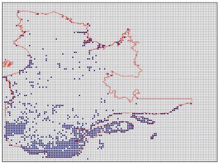
Typically, a heuristic place prioritization algorithm consists of two steps: (i) an initialization step during which a first cell (or set of cells) is selected to initiate the construction of a CAN; and (ii) an iterative step during which a CAN is augmented, cell by cell, until all targets are met. Any of the heuristic rules described above — and many others which have not been mentioned here — may be used at the initialization step. However, in practice, the process will often be initialized using an existing CAN, for instance, the current network of parks, reserves, and other protected areas. The iterative step involves the systematic use of the heuristic rules, and these are often used hierarchically. For instance, rarity may be used first, with ties being broken by complementarity.^[35] Besides the representation of surrogates, other criteria included in Stage 5 (of the framework presented in Section 2) may also be incorporated as heuristic rules for use at this stage. For instance the average size of conservation areas may be increased, and network connectivity encouraged, by introducing a preference for cells adjacent to those already selected when ties are broken between cells that have identical complementarity and rarity values (Nicholls & Margules 1993). Figure 1.1 shows a solution for the ESSCP for Québec; Figure 1.2 for the MESCP.

A heuristic algorithm typically terminates when a “local optimum” is encountered, that is, when the rule being used does not find a better solution at the next step. A meta-heuristic algorithm: (i) controls the execution of a simpler heuristic method; and (ii) unlike a simple heuristic, does not automatically terminate once a locally optimal solution is found. Rather it continues the search process, examining less optimal solutions, while keeping track of the best solution so far found. Meta-heuristic algorithms have two advantages over heuristic ones: (i) they usually produce more optimal solutions, especially when they are initialized with the best solution of a heuristic algorithm; and (ii) typically, meta-heuristic algorithms produce a suite of equally good solutions with no added computational cost (unlike a heuristic algorithm which would have to be executed to obtain each such solution, one at a time). So far, simulated annealing has been the only meta-heuristic algorithm to be systematically used to refine the results of heuristic algorithms for the CAN selection problem.^[36] Recently, a potentially more powerful meta-heuristics, tabu search, has shown great promise (Okin 1997; Pappas et al. 2004).

This discussion of place prioritization has so far assumed that adequate complete sets of cells must be selected simultaneously (that is, in one step). This assumption, until recently shared by virtually all theorists in conservation biology, probably reflects a political naiveté that assumes that all that scientists must do is to produce a plan (especially if care has been taken to incorporate socio-political and other such constraints explicitly) and that it would be implemented. In practice, no complete CAN identified by systematic methods has ever been implemented. Typically, in those few cases in which implementation has occurred at all, some fraction of the identified cells have been initially put under some conservation plan, sometimes followed by later incorporation of a few other cells.^[37] However, because each cell outside a CAN is typically under a different level of threat compared to a cell in a CAN, the optimization problems described above cannot be presumed to capture — and, in some case, can provably be shown not to capture — the problem of prioritizing cells if they are going to be sequentially incorporated in a CAN over a (discretized) period of time, the so-called time horizon of the problem.

This lead to the conservation action scheduling (CAS) problem: select a limited number of cells now, given present knowledge of threats and costs, such that the representation of biodiversity is maximized (as defined for the ESSCP and MESCP) at the end of the time horizon. It is likely that most fully formalized versions of this problem can be optimally solved using backward recursion, for instance, through stochastic dynamic programming.^[38] However, the computational space (available memory) and time complexity of these methods are so extreme as to dwarf those of the optimal algorithms for the ESSCP and MESCP (which were already NP-hard). No plausible heuristic or meta-heuristic algorithm for the CAS problem is so far known — devising one would not go unnoticed.

Figure 1.1
ESSCP Solution for Québec

This figure shows a solution of the ESSCP for Québec using a heuristic place prioritization algorithm initialized by rarity, and using rarity and complementarity sequentially at the iterative step. Ties were broken by adjacency, leading to a preference for larger individual conservation areas. Redundant cells (those cells which can be removed without any surrogate falling short of its target) were removed at the end. This algorithm was incorporated in the ResNet software package (Garson et al. 2002b) which was used for this analysis. 496 species were used as surrogates; the target was set at 90 % of the total expected surrogate coverage for 387 species at risk, and 10 % of the total expected surrogate coverage for the 109 other species for which there were data. This data set was used by Sarakinos et al. (2001) to produce a CAN for Québec. The analysis was done on a 0.05° × 0.05° scale of longitude and latitude. 2 175 cells had data. The total area of the CAN is 96684.9 km.², which is 6.35 % of total area of Quebec. The selected cells are shown in blue.

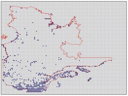
Figure 1.2
MESCP Solution for Québec

The same data set and other parameters were used as for Figure 1.2, except as noted here. The targeted area was set to 10 % of the total area of Québec. All surrogate targets were set at 100 % to allow selection of cells in order of their biodiversity content until the area target was met. The selected cells are shown in blue.

4. Surrogacy

Even though the protection of biodiversity is the explicit goal of conservation biology, the concept of biodiversity has proved notoriously difficult to define (see the entry on biodiversity). It is probably uncontroversial to state that the intended scope of “biodiversity” is biological diversity at every level of structural and functional organization. The problem of using this consensus to produce a definition of biodiversity is that it would include all of biology and, further, such a definition would be impossible to operationalize for the practice of conservation planning. (Because the representation and adequate management of biodiversity is an explicit goal of conservation planning, operationalization of “biodiversity” is a necessity and not a luxury motivated by some recondite philosophical agenda.) Consequently, “surrogates” must be chosen to represent biodiversity. Surrogacy is a relation between a “surrogate” or “indicator” variable and a “target” or “objective” variable.^[39] The surrogate variable represents the objective variable in the sense that it stands in for the latter in the analyses that form part of conservation planning (that is, the former replaces the latter in these analyses). To be of practical use all surrogates must satisfy two criteria (Williams et al. 1994); (i) quantifiability — the variable in question can be measured; and (ii) estimability — it is realistic to assume that the quantified data can be obtained, given constraints on time, expertise, and costs required for data acquisition.

Ultimately, the intended objective variable for all surrogates is biodiversity in general. However, because general biodiversity has so far proven impossible to define adequately, it is useful to distinguish between “true surrogates” and “estimator surrogates.”^[40] True surrogates are supposed to represent general biodiversity. The only formal constraint on a true surrogate set is that it must be amenable to sufficiently precise quantification to carry out place prioritization. The absence of a consensus on the definition of biodiversity makes the designation of any surrogate set as the true surrogate set open to question. Moreover, empirical considerations alone will not allow a resolution of this issue: empirical arguments can only settle questions about relations between empirically well-specified entities. In choosing true surrogates, conventions must enter into the considerations but this does not mean that the choices are arbitrary. These conventions must be justified on grounds of plausibility. Three types of plausible true surrogate sets have most commonly been proposed:

1. character or trait diversity^[41] the customary argument for this choice is that evolutionary mechanisms usually impinge directly on traits of individuals in populations (see the entries on evolutionary genetics; natural selection). The trouble is that “trait” is not a technical term in biology and may be defined in a variety of ways to generate a possibly intractable heterogeneity^[42] consequently, it is unclear that trait diversity is precise enough for place prioritization;
2. species diversity: this can be made sufficiently precise using a wide variety of measures, for instance, the Shannon and Simpson indices.^[43] It is the true surrogate most commonly invoked in discussions of biodiversity conservation, though often only implicitly. Its attractiveness lies in the fact that “species” is the most well-defined category above the genotype in the biological taxonomic hierarchy. The major limitation of using species as true surrogates is that there is obviously much more to biological diversity than species diversity;
3. species assemblage, or landscape pattern, or life-zone diversity: these terms are used in different parts of the world by biologists to mean similar things, though the spatial scale may vary.^[44] They reflect the intuitions that: (a) what is important is the variety of biotic communities with their associated patterns of interactions; and (b) focusing on communities will ipso facto take care of species since communities are composed of species. The chief disadvantage is that, at least on the surface, quantification seems to be impossible: any classification of communities seems to involve arbitrary choices (see the entry on ecology). Life-zone classification produces a partial solution: it involves coupling some characteristics of some communities at a place (in particular, vegetation) with quantifiable environmental parameters such as elevation, precipitation, and temperature (and, sometimes, soil types). For some areas of the world, for instance, Australia (Christian & Stewart 1968; Laut et al. 1977; Thackway and Cresswell 1995) and Costa Rica (Holdridge 1967) precise classifications have been developed.

In contrast to true surrogates, estimator surrogates have true surrogates as their intended objects of representation. Given that a true surrogate set has been precisely delineated (even if only by convention), whether an estimator-surrogate set adequately represents a true surrogate set is an empirical question. Consequently, the adequacy of putative estimator surrogate sets must be established using field data.^[45] How the appropriate concept of representation should be explicated will occupy much of the rest of this section. Meanwhile, note that there is a wide variety of potential estimator surrogate sets including, but not limited to:

1. environmental parameter composition: the theoretical motivation for this choice is the expectation that each point of the space spanned by environmental parameters is a potential niche to be occupied by some species.^[46] The distribution of environmental parameter sets is trivially quantifiable. What makes the use of environmental parameters most attractive is that their distributions are easily obtained from models (for instance, digital elevation models [DEMs], climate modeling based on DEMs, etc.) and using remote-sensed data (from satellite imagery);
2. vegetation classes: vegetation types represent various combinations of species and the interactions between them. Vegetation types also interact with, and provide habitat for, many inconspicuous organisms such as nematodes, arthropods, fungi, protozoa, and bacteria, which may otherwise be missed in conservation planning using other surrogates. The distribution of vegetation classes can not only be easily quantified, but also inferred from remote-sensed data;
3. sub-sets of species composition: species sub-sets such as mammals, birds, plants, butterflies, etc., and combinations of these, are the most easily recognized and widely represented estimator surrogate sets. Data on their distributions can be obtained form surveys. Less satisfactorily, they can be compiled from museums, herbaria, etc.; data from these sources suffer severe problems of spatial bias, with collecting sites often mapping road networks (Margules & Austin 1994), although statistical data treatments are available for partial reduction of such biases (Margules et al. 1995; Hutchinson et al. 1996; Austin & Meyers 1996; Hilbert & van den Muyzenberg 1999).
4. sub-sets of genus or higher taxon composition: these can be used in the same way as sub-sets of species, with data obtained from the same sources and suffering from the same problems.

The use of estimator surrogates rests on an (usually implicit) assumption that there is a model linking the estimator surrogate set and the components of biodiversity that form the true surrogate set. The surrogacy problem consists of demonstrating the adequacy of an estimator-surrogate set, given a true surrogate set. Any method used to demonstrate such adequacy must presume that, for some suitably randomized sub-set of a region (that is, randomized in the space spanned by the parameters representing the proposed estimator surrogates), both the true and estimator surrogate distributions are known. Should an adequate estimator surrogate set be found, it can then be used for conservation planning for the entire region without any further effort being expended to obtain true surrogate distributional data. Of the many methods have so far been proposed for the purpose of establishing adequacy, four are most important:

1. niche modeling: the distributions of estimator surrogates can be used to predict the distributions of true surrogates. The adequacy of the former is measured by the success of such predictions. If species or subsets of species are taken as the true surrogates, methods for such predictions vary from use of sophisticated ecological models to the use of statistical correlations, and includes attempts to use neural networks and genetic algorithms to identify associations.^[47] Until recently few of these methods have been predictively successful.^[48] Moreover, since they generally compute distributions one surrogate (usually species) at a time, they are as yet computationally too intensive for wide-spread adoption in conservation planning which often requires the use of 10³ or more surrogates (as noted in Section 3);
2. species accumulation curves^[49] as a CAN is iteratively constructed using the estimator surrogates, the number of true surrogates represented in it is plotted against the number of selected cells. This plot is compared to: (a) the accumulation of species when sites are iteratively selected using the true surrogates and the same algorithm; and (b) the accumulation when cells are selected at random. The adequacy of an estimator surrogate set is measured by the closeness of the estimator curve is to (a), and its distance from (b);^[50]
3. surrogacy graphs^[51] a potential CAN is iteratively constructed using various combinations of estimator surrogates and targets. The proportion of true surrogates that satisfy their targets (which may differ from each other, and from those set for the estimator surrogates) is plotted against: (a) the proportion of the estimator surrogates that meet their targets; or (b) the proportion of the total area that has so far been selected for inclusion in a CAN. (Both curves are compared to the performace of random selection of cells, as in method [ii].) The goal is to find the smallest subset of estimator surrogates and associated targets such that: (a) either 100 % of the true surrogates satisfy their targets by the time that all the estimator surrogates meet their targets; or (b) these targets are met in as small an area as possible. Figure 4.1 shows a surrogacy graph using environmental parameters in an estimator surrogate set and plant species as the true surrogate set in an area of tropical Queensland;
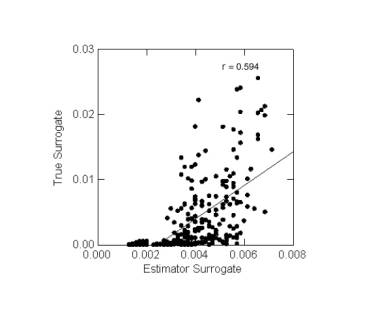
4. marginal contribution plots: for both the true and the estimator surrogates, the relative (or marginal) contribution of each cell to surrogate targets is individually plotted in a graph. The strength of the correlation between the true and estimator surrogate contributions measures surrogate set adequacy. Typically no strong correlation of this sort has been found even when estimator surrogate sets are judged adequate by the second and third methods. The correlation required by this method may be too strong a test for surrogate set adequacy. However, this method has the advantage that it does not rely on targets of representation for surrogates (recalling that these targets are adopted partly by convention). Figure 4.2 shows a marginal contribution graph for one of the estimator surrogate sets tested and found to be adequate in Figure 4.1.

Surrogacy analysis has so far only been poorly explored in conservation biology and whether there are adequate estimator surrogate sets for most true surrogate sets remains an open question. It is generally believed that there are no good biological estimator surrogate sets consisting of lists of species or other taxa; these include the traditional “indicator” species such as keystone, umbrella, and focal species.^[52] The use of environmental surrogate sets appears to be more promising, as does the use of species associations such as vegetation classes.

Figure 4.1
Surrogacy Graph for Queensland

A region of Queensland was divided into cells on a 0.1° × 0.1° scale of longitude and latitude, resulting in 251 cells with an average area of 118 km.² The true surrogate set consisted of 2 348 plant species (195 families). Four estimator surrogate sets were used, based on soil type (2 categories), mean annual temperature (10 categories), maximum temperature during the hottest quarter (4 categories), minimum temperature during the coldest quarter (4 categories), mean annual precipitation (10 categories), elevation (10 categories), aspect (9 categories), and slope (5 categories). In estimator surrogate set 1, all 54 categories were used, in set 2 slope was dropped, in set 3 aspect was also dropped, in set 4 elevation was also dropped. “Random” refers to the coverage of true surrogates if cells are selected at random. The bars refer to the standard deviations (not the standard error) from 100 randomized place prioritization runs using ResNet (Garson et al. 2002b). The graphs record the percentage of the true surrogates captured with a 10 % target of representations as a function of the percentage of the area selected in a CAN. It is clear that all estimator surrogate sets perform much better than random and come close to achieving a 100 % representation of the true surrogates.

Figure 4.2
Marginal Representation Plot for Queensland ES Set 1 at 0.10° Scale

This plot corresponds to the estimator surrogate set 1 in Figure 4.1. The low value of r indicates a poor (though positive) correlation.

5. Vulnerability and Viability

The fact that a cell has a high biodiversity content at present does not guarantee that the biodiversity content of that cell will remain high in the future. The biotic features of a cell may be in decline, sometimes irreversibly so. This possibility raises a fundamental problem for conservation biology: conservation planning must have as its goal the future representation of features, not merely their present representation in CANs. Achieving this goal requires the assessment of the prognosis for biodiversity features in the cells in which they now occur, that is, the viability of these features. The set of cells prioritized for inclusion in a CAN must be refined on the basis of such an assessment. The status of a cell after such an assessment determines its biodiversity value (Sarkar 2002) to be distinguished from its present biodiversity content, as determined by the initial place prioritization (see Section 3). In general, with an important exception which will be discussed in the next paragraph, cells with poor prognosis for biodiversity should be excluded from potential CANs.

However, the prognosis for biodiversity in a cell will depend on the management plan for that cell. Cells with the highest biodiversity value are those with high biodiversity content that have a favorable prognosis for their biodiversity under minimal management plans, that is, plans that require the least additional knowledge or effort to implement. Nevertheless, cells may sometimes have high biodiversity value even if the present prognosis for their biodiversity content is grim provided that the represented biodiversity features are irreplaceable elsewhere. (For instance, a cell with degraded habitat may contain the last population of a critically endangered species.) In such a circumstance, conservation planning calls for the formulation and implementation of adequate management plans even if the process is fraught with practical difficulty and uncertainty. (This is where the recently-formulated program of restoration ecology may have much to contribute to conservation biology.) Such cells must be deemed as having high biodiversity value despite the poor present prognosis for their biodiversity content.

Unfortunately, the problem of assessing the prognosis of biodiversity under various management plans remains poorly understood, both theoretically and experimentally. This problem is typically called “viability analysis” in North America (and known by a variety of names including “vulnerability analysis” elsewhere). In retrospect, the early attempts to use island biogeography theory to determine the prognosis for biodiversity at a place from its area (see Section 1) constituted a rudimentary viability analysis based on community ecology (see the entry on ecology). The failures of those attempts led to a shift of attention to population ecology. The result was population viability analysis (PVA) (Boyce 1992). As noted in Section 1, no generally accepted framework for PVA has yet emerged. Even if an adequate framework should emerge — and the present prospects seem dim — it is at least questionable how valuable PVA can be for systematic conservation planning.

PVAs can only be performed for single species (and, usually, single populations) or a very few species at a time. When the prognosis for hundreds of species must be simultaneously determined, PVA is practically useless.^[53] This criticism should not be misinterpreted to suggest that PVAs have no valuable role to play in conservation planning. When conservation plans have to be devised for individual species of obvious importance — for instance, phylogenetically uncommon endangered species — adequate PVAs may well be critical for planning purposes. However, even here, technical limitations of PVAs — at least as they have so far been performed — pose problems. Models for PVA have proven to be notoriously susceptible to two problems: (i) partial observability — even simple parameters such as the intrinsic growth rate of a population or the carrying capacity of a habitat are almost intractably difficult to estimate with requisite precision from field data (Shrader-Frechette & McCoy 1993; Sarkar 1996a) and (ii) structural uncertainty — apparently slightly different models of the same biological situation make radically different predictions. This phenomenon has been observed for almost all simulation and analytic models used for PVA. One solution has been to suggest that PVA should not be used to make absolute predictions about parameters such as the expected time to extinction. Rather, it should be used to rank different management plans for the same population when all models produce the same ranking.^[54] Alternatively, it can similarly be used to rank different populations under the same management plan, once again when all models produce the same ranking.

Given the difficulties faced by PVA, much effort is currently being expended towards developing methodologies for assessing the prognosis for the full complement of biodiversity at a place. These methods have usually been classified into three categories (Durant & Mace 1994; Gaston et al. 2002) (i) subjective assessments; (ii) heuristic rules which are supposed to be an advance over purely subjective assessments; and (iii) quantitative risk modeling, which includes traditional PVA as a particularly simple (or degenerate) case. All three methods are being applied to single taxa (obviously including species), sets of taxa, and, most importantly, to entire habitats. At present, all of these methods (except traditional PVA) remain rudimentary. These methods also underscore the extent to which conservation biology must diverge from traditional (or purely scientific) ecology. Subjective assessments usually do not form part of a science, and even the use of heuristic rules is rare. Both of these types of methods routinely draw on socio-political knowledge, for instance, whether a species is being harvested at a high rate (which increases its risk of extinction). Even quantitative risk modeling often requires moving beyond the biological sciences in to the social sciences, with their attendant problems of interpretation and prediction.

For individual taxa, one important use of vulnerability assessment has been to set targets of representation for biodiversity in CANs. All three types of method have been used for this purpose. Most designations of taxa as being at high risk of extinction are based on subjective assessments or only slightly more formal heuristic rules (Munton 1987; Gaston et al. 2002). Typically, very high targets are set for such surrogates when CANs are selected. For instance, Sarakinos and several collaborators set a target of 100 % for most species at risk while formulating a plan for Québec (Sarakinos et al. 2001). Kirkpatrick and Brown have used modeled risk assessment to set targets as high as 90 % of the pre-European extent for some vulnerable or rare vegetation types in New South Wales (Kirkpatrik & Brown 1991).

However, a much more important use of vulnerability assessments is to refine CANs. For instance, Cameron produced 100 alternative CANs to represent 10 % of 46 vegetation types (the estimator surrogates) in continental Ecuador.^[55] Two heuristic rules were used to assess vulnerability: (i) distance to an anthropogenically transformed area, which was taken to be strongly correlated with the threat of habitat conversion; and (ii) distance form a reserve which was taken to increase the viability of the biota of a cell. The set of CANs was then refined to incorporate these rules using a method of multiple criterion synchronization discussed in the next section.

6. Multiple Criterion Synchronization

Attempts to conserve biodiversity always take place in contexts in which there are many other competing claims for the use of land (as discussed at the beginning of 3). With the exception of perhaps limited (sometimes called “sustainable”) recreation and biological resource extraction, these other uses are almost always incompatible with biodiversity conservation. In the 1980s, conservation biologists, particularly in North America, drawing on a variety of ethical doctrines such as “deep ecology” (see Environmental Ethics) summarily condemned these other uses as being ethically inferior to biodiversity conservation. This position found little support outside affluent societies (of what is often called the “North” in environmental politics even though it includes nations such as Australia and New Zealand).^[56] When alternative uses of land are necessary for human survival, as it often is in impoverished societies (which are impoverished largely as a result of European and neo-European colonialism), strictures against such uses of land carry little ethical weight. Beyond such ethical reasons, by the early 1990s, conservation biologists also began to recognize that there are compelling prudential reasons for not ignoring human interest in other uses of land when conservation policies have to be devised. A salutary example was India's Project Tiger. Launched in the 1970s to protect endangered populations of Panthera tigris tigris in southern Asia, Project Tiger largely consisted of the creation of tiger reserves by the expulsion of human residents of habitats. Initially proclaimed as a major conservation success as tiger populations allegedly increased, it was recognized as a failure in the 1980s largely because of illegal hunting. These hunters managed to operate with impunity in the forests partly because of local support from displaced residents (Gadgil & Guha 1995).

Permitting consideration of alternative uses of land provided the impetus for the incorporation of multicriteria decision making (MCDM) in conservation biology. The problem is usually conceived of as the simultaneous optimization of multiple criteria such as the various uses of land and also other, biologically relevant criteria, such as those incorporating vulnerability and threat (see Section 5). However, as the methods discussed below will show, there is no mathematical sense in which the various criteria are being optimized. This is the reason why these procedures are being called "multiple criterion synchronization" here.^[57] The crucial philosophical question is whether these different criteria should be regarded as commensurable (in the sense of being reducible to the same scale). The last decade has seen many attempts to carry out multiple criterion synchronization without assuming such commensurability (see below).

There are three methods that have commonly been used to attempt to resolve problems involving the use of multiple criteria in conservation planning:

1. reduction to a single utility function: this method originates in neoclassical economics where it is assumed that all values can be assessed on a single quantitative scale of utility (or cost). This utility is supposed to be measured by agents' preferences which can be estimated by what they are willing to pay for these values or the compensation they require to give them up. There are many conceptual and empirical problems associated with this approach. Perhaps the most important conceptual problem is that this method assumes that all the relevant values are commensurable (that is, they can be quantitatively assessed on the same scale). Empirical problems include the difficulty of carrying out willingness-to-pay (WTP) estimation and similar assessments as well as the intransitivity and temporal instability of such preferences (Norton 1987, 1994). Whatever be the merits or problems associated with such uses of preferences, in practice in environmental contexts, systematic WTP or other assessments are almost never carried out because of operational difficulties. Rather, specific utility functions are usually chosen using educated intuition and partial information elicited from agents. In environmental contexts this method has most credibly been used to assess the value of ecosystem services for comparison with the value of forgone economic opportunities when an ecosystem is left undeveloped.^[58] However, since systematic WTP and similar assessments were not carried out, such exercises are open to charges of arbitrariness. As a result, in recent years, most attempts to develop systematic methods for environmental decision evaluation have turned to more sophisticated analyses;
2. reduction to a parameterized utility function with accompanying sensitivity analyses: this method also involves using an utility function, but each additive component of that function represents a different criterion with an associated weight. These weights are used in sensitivity analyses. Suppose that a set of alternatives is ranked using this utility function with one set of weights. Each weight can then be varied across its entire range to test the invariance of the ranking. High invariance indicates a high reliability of the ranking. More importantly, the weights can be used to analyze trade-offs between the criteria. In the context of CAN design, this method has been advocated by Faith and used in several contexts, including Papua New Guinea (Faith 1995; Faith et al. 2001).
3. identification of a set of non-dominated alternatives, sometimes followed by further refinement of that set:^[59] the third method explicitly eschews any attempt to compare different, potentially incommensurable, criteria on the same scale. It starts with two structures, a set of criteria, Κ = {κ_i | i = 1, 2, … , n}, and a set of feasible alternatives, Α = {α_j | j = 1, 2, … , m}. It is assumed that each criterion κ_i induces a weak linear order ≤_i^* on Α, that is, for ∀κ_i ∈ Κ and ∀α_j,α_k,α_l ∈ Α, α_j≤_i^*α_k, or α_k≤_i^*α_j or both; if α_j≤_i^*α_k and α_k≤_i^*α_l, then α_j≤_i^*α_l (that is, ≤_i^* is transitive). Each ≤_i^* thus imposes an ordinal structure on Α giving ranks to the α_j (j = 1, 2, … , m). However, since the order is only weak, two different alternatives may have the same rank. Let ν_ij be the rank of alternative α_j by the criterion κ_i. For all alternatives, α_e and α_f, e ≠ f, α_e dominates α_f or α_f α_f if and only if:
   
   

   ∃i(ν_ie < ν_if) & ∀k(ν_ke ≤ ν_kf).

   Therefore, for all alternatives, α_e and α_f, e ≠ f, α_e does not dominate α_f or ¬(α_f α_f) if and only if:

   ¬(∃i(ν_ie < ν_if) & ∀k(ν_ke ≤ ν_kf))

   ⇔ ¬∃i(ν_ie < ν_if) ¬∀k(ν_ke ≤ ν_kf)
   ⇔ ∀i¬(ν_ie < ν_if) ∃k¬(ν_ke ≤ ν_kf)
   ⇔ ∀i¬(ν_ie < ν_if) ∃k(ν_ke ≤ ν_kf)

   It is assumed, by convention, that ¬(α_e α_e). Thus, if α_i dominates α_j, there is no criterion by which α_j can be regarded as better than α_i because α_j is never ranked lower than α_i. The set of "non-dominated" alternatives consists of those alternatives that are not dominated by any alternative. Note that the determination of non-dominated alternatives does not involve comparing different criteria, let alone attempting to reduce them to one scale. Using this method, Rothley (1999) identified 36 CANs for Nova Scotia and then found non-dominated solutions for cost and area by visual inspection; the logical relations noted above are due to Sarkar and Garson ( 2004). Figure 6.1 shows an example from Ecuador where this process has been carried out.

The obvious value of the third method is that the sense in which non-dominated alternatives are better than dominated ones involves no arbitrary ranking of the criteria or any other ad hoc assumption. Moreover, all non-dominated solutions are “equally optimal” in the sense that there is no available information on the basis of which one can be judged better than another. In the planning process the set of non-dominated solutions is presumed to be presented to decision-makers with an “expert opinion” to the effect that exact (non-arbitrary) systematic methods can go no further. The decision-makers can then bring into play those socio-economic or biological factors that were not modeled in the analysis (or other even less tangible politically relevant factors). That there will generally be more than one non-dominated solution is a virtue because the availability of several “equally optimal” options allows flexibility in the ensuing decision-making process.

However, typically, the number of non-dominated solutions increases with the number of criteria and the non-dominated set is often intractably large. In such cases, the third method cannot be used as it stands: a method that presents scores of alternatives to planners will often be practically usesless. The only option at this point is to refine the non-dominated set further, by introducing a ranking of the non-dominated alternatives, for instance, by ranking the criteria. A wide variety of methods have been developed for this purpose^[60] and probably each has its advocates in conservation planning. At present, the Analytic Hierarchy Process appears to be one of the more popular of such methods (Anselin et al. 1989; Kuusipalo & Kangas 1994; Li et al. 1999; Villa 2001). However, every such method that is known has at least some ad hoc assumptions built into it and there is nothing like an emerging consensus about the best MCDM protocol for use in conservation planning.

Figure 6.1
MCS Plot for Ecuador

Cameron (2003) generated 100 CANs for Ecuador using 46 vegetation types as surrogates and a target of 10 % for each using the ResNet software package (Garson et al. 2002b). Multiple criterion synchronization was then carried out to minimize the area to an existing reserve while maximizing the distance to a transformed area. Multiple criteria: x-axis: compounded (summed) distance from a reserve; y-axis: compounded distance from anthropogenically transformed areas. The non-dominated solutions are those that have no other alternatives to the left or to the bottom of them. They are shown in red.

7. Final Remarks

Conservation biology emerged as a recognizable science within the last two decades. It has provided philosophers of science (as well as historians and sociologists) with a rare opportunity to observe a discipline during the process of its formation. Philosophical scrutiny of conservation biology began with the work of Norton and Shrader-Frechette in the late 1980s and early 1990s and has continued to the present day (Norton 1987; Shrader-Frechette 1990; Shrader-Frechette & McCoy 1993, 1994). At the most general epistemological level, four themes have emerged which have already been introduced in this entry. These final remarks will explicitly connect these themes with more traditional philosophical issues and terminology:

1. the adoption of conventions has been central to many developments, including the setting of targets for the representation of biodiversity in CANs and the choice of surrogates. The adoption of conventions has involved public discussion and debate, as should be expected: conventionality does not mean arbitrariness. There are good reasons for some conventions; not for others. Many conventions, such as the targets mentioned in Section 2, remain controversial. Others, such as using all species as true surrogates for biodiversity, already have an aura of authenticity. As these conventions begin to get reified by inclusion in textbooks and other summaries, they may eventually appear to be “real” in the sense that they appear to be facts about biodiversity rather than conventions adopted for pragmatic reasons. On the one hand, conservation biology may be unique among the sciences with respect to such a reliance on conventions. On the other hand, what appears to be happening in conservation biology may well be characteristic of scientific discipline-formation in general. To the extent that the latter generalization is correct, this aspect of discipline-formation provides a compelling argument against realism in the interpretation of scientific theories;
2. practically unavoidable exigencies, for instance, the requirement that a multiple synchronization process return a limited number of final alternatives has the potential to require a tolerance of ad hoc procedures. In some ways these are similar to conventions but the dissimilarities are more important: in particular, there is even less justification for these ad hoc procedures than there is for most conventions. Yet, because of pragmatic reasons, they may be unavoidable. Such a development would argue for a more pragmatic (or instrumentalist; again, in contrast to a realist) attitude towards science;
3. from the estimation of ecological parameters and assessments of vulnerability to the prediction of results of conservation plans, conservation biology is unique in the extent to which it is riddled with the problem of coping with uncertainty. This has led many researchers to predict that a Bayesian future lies ahead for conservation biology because only a Bayesian framework allows the seamless concatenation of the results of experiments and models with decision-making protocols.^[61] Whether or not a Bayesian framework proves indispensable, it is almost certainly true that the development of reliable conservation plans will require a far more systematic treatment of uncertainty than what has so far been attempted. There is exciting epistemological work to be done in this area, one in which philosophy has much to contribute to science;
4. several areas of conservation biology, in particular, multiple criterion synchronization, serve as a reminder that both scientific research and practical decision making operate under the constraint of bounded rationality. There is no uncontroversial unique measure of biodiversity. Heuristic methods must be used because optimal methods are intractable, given the temporal constraints on decision-making. Alternative conservation plans must be ordered according to criteria that, at least initially, appear to be intangible. The intransitivity of preferences must be negotiated. Decisions must yet be made, not only under uncertainty (as discussed in [iii] above), but within limited time periods. Any philosophical progress in clarifying and “rationalizing” these processes will have important practical consequences for conservation biology.^[62]

Turning to issues more internal to conservation biology, four other themes have emerged:

1. the first lesson to draw from the discussion above is the extent to which conservation biology has diverged from traditional ecology (see the entry on ecology). The only part of the consensus framework that falls squarely within traditional ecology is population viability analysis and this has arguably been, to date, the least successful part of conservation biology. In particular (as noted in Section 3), the constraint that conservation biology must necessarily embrace the particularities of individual places distinguishes it from ecology. The distinction that is thus introduced is philosophically important: while conservation biology may utilize reliable generalizations from ecology (when available), it does not usually expect to find universal principles in the form of “laws” and “theories” (as philosophers use those terms) applicable to all places.^[63] Ecology, in contrast, is yet to give up the hope for such principles;
2. conservation biology has emerged as a hybrid discipline with techniques drawn from a variety of sources including computer science, the geosciences, and the social sciences.^[64] The importance of the social sciences — mainly because, biodiversity conservation necessarily takes place in a socio-political context — is only likely to increase in the future. In fact it may soon be the case that the question that will have to be asked is that, beyond the mere inventory of biota, that is, biogeography, what biology per se has to contribute to conservation science. Is conservation biology ultimately a social science?;
3. part of the skepticism about the role of biology in conservation science is engendered by the early experience of conservation biology, when simplistic applications of biological theory to the problems of conservation science, for instance, the use of island biogeography theory to design nature reserves, proved to be unmitigated failures (recall the discussion of Section 1). However, recent developments within ecology, for instance, individual-based models, restoration ecology, spatial ecology, and landscape ecology, may well finally produce a body of robust ecological knowledge that is uncontroversially applicable to biodiversity conservation in the field. These may transform the field. Ecology itself has been transformed during the last few decades (see ecology), and it is at least plausible to argue that both fields are partly converging to a set of models and techniques which will help unify them;
4. perhaps most interestingly, as already noted in Section 3, what constitutes theory in conservation biology are not the typical descriptive laws summarizing phenomena, but, rather, algorithms designed to help the decision-making process in highly localized (and possibly idiosyncratic) contexts. To the extent that conservation biology seeks universality, it is at the level of these algorithms. An exploration of what this sense of “theory” is falls beyond the scope of this entry though it merits more philosophical reflection.^[65] Suffice it here to note that conservation biology is analogous in this respect to some other applied goal-oriented “sciences,” in particular, medicine.^[66] It may well be the case that the future will see many more sciences with algorithms as theories and the most valuable science will consist of constructing highly contextual procedures rather than producing general theories usually preferred by traditional philosophers of science.

Bibliography

• Ackery, P. R. and Vane-Wright, R. I. 1984. Milkweed Butterflies. Ithaca, NY: Cornell University Press.
• Andelman, S. J. and Fagan, W. F. 2000. “Umbrellas and Flagships: Efficient Conservation Surrogates, or Expensive Mistakes?” Proceedings of the National Academy of Sciences (USA) 97: 5954 -5959.
• Anselin, A., Meire, P. M., and Anselin, L. 1989. “Multicriteria Techniques in Ecological Evaluation: An Example Using the Analytical Hierarchy Process.” Biological Conservation 49: 215 -229.
• Araújo, M. B., Densham, P. J., and Humphries, C. 2003. “Predicting Species Diversity with ED: The Quest for Evidence.” Ecography 26: 380 -383.
• Araújo, M. B., Densham, P. J., Lampinen, R., Hagemeijer, W. J. M., Mitchell-Jones, A. J. and Gase, J. P. 2001. “Would Environmental Diversity Be a Good Surrogate for Species Diversity?” Ecography 24: 103 -110.
• Austin, M. P. and Meyers, J. A. 1996. “Current Approaches to Modelling the Environmental Niche of Eucalypts: Implications for Management of Forest Biodiversity.” Forest Ecology and Management 85: 95 -106.
• Ball, I. R. 2000. “Mathematical Applications for Conservation Ecology: The Dynamics of Tree Hollows and The Design of Nature Reserves.” PhD Thesis, The University of Adelaide.
• Berry, D. A. 1996. Statistics: A Bayesian Perspective. Belmont, MA: Duxbury.
• Boyce, M. S. 1992. “Population Viability Analysis.” Annual Review of Ecology and Systematics 23: 481 -506.
• Callicott, J. B. and Nelson, M. P. Eds. 1998. The Great New Wilderness Debate. Athens, GA: University of Georgia Press.
• Cameron, S. 2003. “Place Prioritization and Multiple Criterion Synchronization for Biodiversity Conservation in Ecuador using Modeled Vegetation Classes as Surrogates.” Honors Thesis. Department of Biology, University of Texas at Austin.
• Caughley, G. 1994. “Directions in Conservation Biology.” Journal of Animal Ecology 63: 215 -244.
• Caughley, G. and Gunn, A. 1996. Conservation Biology in Theory and Practice. Boston: Blackwell Science.
• Christian, C. S. and Stewart, G. A. 1968. “Methodology of Integrated Surveys.” In United Nations Educational, Scientific and Cultural Organization. Ed. Proceedings of the Toulouse Conference on Aerial Surveys and Integrated Studies. Paris: UNESCO, pp. 233 -280.
• Csuti, B., Polasky, S., Williams, P. H., Pressey, R. L., Camm, J. D., Kershaw, M., Kiester, A. R., Downs, B., Hamilton, R., Huso, M., and Sahr, K. 1997. “A Comparison of Reserve Selection Algorithms Using Data on Terrestrial Vertebrates in Oregon.” Biological Conservation 80: 83 -97.
• Diamond, J. M. and May, R. M. 1976. "Island Biogeography and the Design of Natural Reserves." In May, R. M. Ed. Theoretical Ecology: Principles and Applications. Oxford: Blackwell, pp. 163-186.
• Durant, S. M. and Mace, G. M. 1994. “Species Differences and Population Structure in Population Viability Analysis.” In Olney, P. J. S., Mace, G. M., and Feistner, A. T. C. Eds. Creative Conservation: Interactive Management of Wild and Captive Animals. London: Chapman and Hall, pp. 67 -91.
• Faith, D. P. 1992. “Conservation Evaluation and Phylogenetic Diversity.” Biological Conservation 61: 1 -10.
• Faith, D. P. 1995. Biodiversity and Regional Sustainability Analysis. Lyneham: CISRO Division of Wildlife and Ecology.
• Faith, D. P. 2003. “Environmental Diversity (ED) as Surrogate Information for Species-Level Diversity.” Ecography 26: 374 -379.
• Faith, D. P., Margules, C. R., and Walker, P. A. 2001. “A Biodiversity Conservation Plan for Papua New Guinea Based on Biodiversity Trade-Offs Analysis.” Pacific Conservation Biology 6: 304-324.
• Faith, D. P. and Walker, P. A. 1996a. “Environmental Diversity: On the Best-possible Use of Surrogate Data for Assessing the Relative Biodiversity of Sets of Areas.” Biodiversity and Conservation 5: 399-415.
• Ferrier, S., Pressey, R. L., and Barrett, T. W. 2000. “A New Predictor of the Irreplacability of Areas for Achieving a Conservation Goal, Its Application to Real-World Planning, and a Research Agenda for further Refinement.” Biological Conservation 93: 303 -325.
• Ferrier, S. and Watson, G. 1997. “An Evaluation of the Effectiveness of Environmental Surrogates and Modelling Techniques in Predicting the Distribution of Biological Diversity: Consultancy Report to the Biodiveristy Convention and Strategy Section of the Biodiversity Group, Environment Australia.” Arimidate: Environment Australia.
• Gadgil, M. and Guha, R. 1995. Ecology and Equity: The Use and Abuse of Nature in Contemporary India. New Delhi: Penguin Books India.
• Garson, J., Aggarwal, A., and Sarkar, S. 2002a. “Birds as Surrogates for Biodiversity: An Analysis of a Data Set from Southern Québec.” Journal of Biosciences 27(S2): 347 -360.
• Garson, J., Aggarwal, A., and Sarkar, S. 2002b. “ResNet Ver 1.2 Manual.” Report. Austin: University of Texas Biodiversity and Biocultural Conservation Laboratory.
• Gaston, K. J., Pressey, R. L., and Margules, C. R. 2002. “Persistence and Vulnerability: Retaining Biodiversity in the Landscape and in Protected Areas.” Journal of Biosciences 27(S2): 361 -384.
• Gilpin, M. E. and Soulé, M. E. 1986. “Minimum Viable Populations: Processes of Species Extinction.” In Soulé, M. E. Ed. Conservation Biology: The Science of Scarcity and Diversity. Sunderland: Sinauer, pp. 19 -34.
• Groves, C. R., Jensen, D. B., Valutis, L. L., Redford, K. H., Shaffer, M. L., Scott, J. M., Baumgartner, J. V., Higgins, J. V., Beck, M. W., and Anderson, M. G. 2002. “Planning for Biodiversity Conservation: Putting Conservation Science into Practice.” BioScience 52: 499 -512.
• Guha, R. 1989. “Radical American Environmentalism and Wilderness Preservation: A Third World Critique.” Environmental Ethics 11: 71 -83.
• Hanski, I. A. 1999. Metapopulation Ecology. Oxford: Oxford University Press.
• Hedrick, P. W., Lacy, R., C., Allendorf, F. W., and Soulé, M. E. 1996. “Directions in Conservation Biology: Comments on Caughley.” Conservation Biology 10: 1312 -1320.
• Hilbert, D. W. and Muyzenberg, J. v. d. 1999. “Using an Artificial Neural Network to Characterize the Relative Suitability of Environments for Forest Types in a Complex Tropical Vegetation Mosaic.” Diversity and Distributions 5: 263 -274.
• Holdridge, L. R. 1967. Life Zone Ecology. San Jose: Costa Rica
• Holling, C. S. Ed. 1978. Adaptive Environmental Assessment and Management. Chichester: Wiley.
• Hubbell, S. P. 2001. The Unified Neutral Theory of Biodiversity and Biogeography. Princeton: Princeton University Press.
• Hutchinson, M. F., Belknap, J. K., Nicholls, A. O., Nix, H. A., McMahon, J. P., and Ord, K. D. 1996. BioRap. Vol. 2. Spatial Modelling Tools. Canberra: CSIRO.
• International Union for the Conservation of Nature (IUCN). 1980. World Conservation Strategy: Living Resource Conservation for Sustainable Development. Gland: International Union for the Conservation of Nature.
• International Union for the Conservation of Nature (IUCN). 1983. Parks and Life: Report of the IVth World Congress on National Parks and Protected Areas. Gland: International Union for the Conservation of Nature.
• Janzen, D. H. 1986. “The Future of Tropical Ecology.” Annual Review of Ecology and Systematics 17: 305 -324.
• Jones, B. D. 1999. “Bounded Rationality.” Annual Review of Political Science 2(1): 297 -321.
• Justus, J. and Sarkar, S. 2002. “The Principle of Complementarity in the Design of Reserve Networks to Conserve Biodiversity: A Preliminary History.” Journal of Biosciences 27(S2): 421 -435.
• Kelly, K. and Glymour, C. 2004. “Why Probability Does Not Capture the Logic of Scientific Justification.” In Hitchcock, C., (ed.), Contemporary Issues in the Philosophy of Science. pp. 94 -114.
• Kingsland, S. 2002. “Creating a Science of Nature Reserve Design: Perspectives from History.” Environmental Modeling and Assessment 7: 61 -69.
• Kirkpatrick, J. B. 1983. “An Iterative Method for Establishing Priorities for the Selection of Nature Reserves: An Example from Tasmania.” Biological Conservation 25: 127 -134.
• Kirkpatrick, J. B. and Brown, M. J. 1991. Reservation Analysis of Tasmanian Forests. Canberra: Resource Assessment Commission.
• Kirkpatrick, S., Gelatt, Jr., C. D., and Vecchi, M. P. 1983. “Optimization by Simulated Annealing.” Science 220: 671-220.
• Kuusipalo, J. and Kangas, J. 1994. “Managing Biodiversity in a Forestry Environment.” Conservation Biology 8: 450-460.
• Landres, P. B., Verner, J., and Thomas, J. W. 1988. “Ecological Uses of Vertebrate Indicator Species: A Critique.” Conservation Biology 2: 316 -328.
• Laut, P., Heyligers, P. C., Keig, G., Löffler, E., Margules, C. R., and Scott, R. M. 1977. Environments of South Australia: Handbook. Canberra: CSIRO Division of Land Use Research.
• Lewontin, R. C. 2000. The Triple Helix: Gene, Organism, and Environment. Cambridge, MA: Harvard University Press.
• Li, W., Wang, Z., and Tang, H. 1999. “Designing the buffer zone of a nature reserve: a case study in Yancheng Biosphere Reserve, China.” Biological Conservation 90: 159 -165.
• Lindenmayer, D. B., Manning, A. D., Smith, P. L., Possingham, H. P., Fischer, J., Oliver, I., and McCarthy, M. A. 2002. “The Focal-Species Approach and Landscape Restoration: A Critique.” Conservation Biology 16: 338 -345.
• MacArthur, R. A. and Wilson, E. O. 1967. The Theory of Island Biogeography. Princeton: Princeton University Press.
• Magurran, A. E. 1988. Ecological Diversity and Its Measurement. Princeton: Princeton University Press.
• Mann, C. C. and Plummer, M. L. 1995. Noah's Choice: The Future of Endangered Species. New York: A. A. Knopf.
• Margules, C. R. 1989. “Introduction to Some Australian Developments in Conservation Evaluation.” Biological Conservation 50: 1 -11.
• Margules, C., Higgs, A. J. and Rafe, R. W. 1982. “Modern Biogeographic Theory: Are There Lessons for Nature Reserve Design?” Biological Conservation 24: 115 -128.
• Margules, C. R., Nicholls, A. O., and Pressey, R. L. 1988. “Selecting Networks of Reserves to Maximize Biological Diversity.” Biological Conservation 43: 63 -76.
• Margules, C. R. and Pressey, R. L. 2000. “Systematic Conservation Planning.” Nature 405: 242 -253.
• Margules, C. R., Redhead, T. D., Faith, D. P., and Hutchinson, M. F. 1995. Guidelines for Using the BioRap Methodology and Tools. Canberra: CSIRO.
• May, R. M. 1975. “Island Biogeography and the Design of Wildlife Preserves.” Nature 254: 177 -178.
• McCarthy, M. A., Andelman, S. J., and Possingham, H. P. 2003. “Reliability of Relative Predictions in Population Viability Analysis.” Conservation Biology 17: 982 -989.
• Meffe, G. K. and Carroll, C. R. 1994. Principles of Conservation Biology. Sunderland, MA: Sinauer Associates.
• Munton, P. 1987. “Concepts of Threat to the Survival of Species Used in Red Data Books and Similar Compilations.” In Fitter, R. and Fitter, M., (ed.), The Road to Extinction: Problems with Categorizing the Status of Taxa Threatened with Extinction. Gland: IUCN, pp. 71 -111.
• Nicholls, A. O. and Margules, C. R. 1993. “An Upgraded Reserve Selection Algorithm.” Biological Conservation 64: 165 -169.
• Nix, H. A. 1982. “Environmental Determinants of Biogeography and Evolution in Terra Australia.” In Baker, W. R. and Greensdale, P. J. M., (ed.), Evolution of the Flora and Fauna of Australia. Adelaide: Peacock, pp. 47 -76.
• Norton, B. G. 1987. Why Preserve Natural Variety? Princeton: Princeton University Press.
• Norton, B. G. 1994. “Economists' Preferences and the Preferences of Economists.” Environmental Values 3: 313 -332.
• Oelschlaeger, M. Ed. 1995. Postmodern Environmental Ethics. Albany: State University of New York Press.
• Okin, W. J. 1997. “The Biodiversity Management Area Selection Model: Constructing a Solution Approach.” M. A. Thesis, University of California, Santa Barbara.
• Pappas, C., Srinivasan, R. K., Barnes, J. W. and Sarkar, S. 2004. “A Comparison of Heuristic, Meta-Heuristic and Optimal Approaches to the Selection of Conservation Area Networks.”
• Peterson, A. T. 2001. “Predicting Species' Geographic Distributions Based on Ecological Niche Modeling.” Condor 103: 599 -605.
• Possingham, H. P., Day, J. R., Goldfinch, M., and Salzborn, F. 1993. “The Mathematics of Designing a Network of Protected Areas for Conservation.” In Sutton, D. J., Pearce, C. E. M., and Cousins, E. A. Eds. Decision Sciences: Tools for Today. Adelaide: ASOR, pp. 536 -545.
• Pressey, R. L., Possingham, H. P., and Day, J. R. 1997. “Effectiveness of Alternative Heuristic Algorithms for Approximating Minimum Requirements for Conservation Reserves.” Biological Conservation 80: 207 -219
• Primack, R. B. 1993. Essentials of Conservation Biology. Sunderland, MA: Sinauer.
• Rebelo, A. G. and Siegfried, W. R. 1990. “Protection of Fynbos Vegetation: Ideal and Real-World Options.” Biological Conservation 54: 15 -31.
• Roloff, G. J. and Haufler, J. B. 1997. “Establishing Population Viability Planning Objectives Based on Habitat Potentials.” Wildlife Society Bulletin 25: 895 -904.
• Rothley, K. D. 1999. “Designing Bioreserve Networks to Satisfy Multiple, Conflicting Demands.” Ecological Applications 9: 741 -750.
• Sarakinos, H., Nicholls, A. O., Tubert, A., Aggarwal, A., Margules, C. R., and Sarkar, S. 2001. “Area Prioritization for Biodiversity Conservation in Québec on the Basis of Species Distributions: A Preliminary Analysis.” Biodiversity and Conservation 10: 1419 -1472.
• Sarkar, S. 1996a. “Ecological Theory and Anuran Declines.” BioScience 46: 199 -207.
• Sarkar, S. 1996b. “Postmodernism and Biodiversity Conservation.” Conservation Biology 10: 305 -306.
• Sarkar, S. 1998a. Genetics and Reductionism. New York: Cambridge University Press.
• Sarkar, S. 1998b. “Restoring Wilderness or Reclaiming Forests?” Terra Nova 3(3): 35 -52.
• Sarkar, S. 1999. “Wilderness Preservation and Biodiversity Conservation--Keeping Divergent Goals Distinct.” BioScience 49: 405 -412.
• Sarkar, S. 2002. “Defining ‘Biodiversity’: Assessing Biodiversity.” Monist 85: 131 -155.
• Sarkar, S. 2003. “Conservation Area Networks.” Conservation and Society 1(2): v -vii.
• Sarkar, S. 2004. Biodiversity and Environmental Philosophy. New York: Cambridge University Press, in press.
• Sarkar, S., Aggarwal, A., Garson, J., Margules, C. R., and Zeidler, J. 2002. “Place Prioritization for Biodiversity Content.” Journal of Biosciences 27(S2): 339 -346.
• Sarkar, S. and Garson, J. 2004. “Multiple Criterion Synchronization (MCS) for Conservation Area Network Design: The Use of Non-Dominated Alternative Sets.”(???)
• Sarkar, S. and Margules, C. R. 2002. “Operationalizing Biodiversity for Conservation Planning.” Journal of Biosciences 27(S2): 299 -308.
• Sarkar, S., Pappas, C., Garson, J., Aggarwal, A., and Cameron, S. 2004. “Place Prioritization for Biodiversity Conservation Using Probabilistic Surrogate Distribution Data.” Diversity and Distributions 10:125 -133.
• Sarkar, S., Parker, N. C., Garson, J., Aggarwal, A., and Haskell, S. 2000. “Place Prioritization for Texas Using GAP Data: The Use of Biodiversity and Environmental Surrogates within Socioeconomic Constraints.” Gap Analysis Program Bulletin 9: 48 -50.
• Scott, J. M., Heglund, P. J., Morrison, M. L., Haufler, J. B., Raphael, M. G., Wall, W. A., and Samson, F. B. Eds. 2002. Predicting Species Occurrences: Issues of Accuracy and Scale. Washington: Island Press.
• Shafer, C. L. 1999. “National Park and Reserve Planning to Protect Biological Diversity: Some Basic Elements.” Landscape and Urban Planning 44: 123 -153.
• Shaffer, M. L. 1978. “Determining Minimum Viable Population Sizes: A Case Study of the Grizzly Bear.” Ph. D. Dissertation, Duke University.
• Shrader-Frechette, K. 1990. “Island Biogeography, Species-Area Curves, and Statistical Errors: Applied Biology and Scientific Rationality.” In Fine, A., Forbes, M., and Wessels, L. Eds. PSA 1990: Proceedings of the 1990 Biennial Meeting of the Philosophy of Science Association. 1. East Lansing: Philosophy of Science Association, pp. 447 -456.
• Shrader-Frechette, K. S. and McCoy, E. D. 1993. Method in Ecology: Strategies for Conservation. Cambridge, UK: Cambridge University Press.
• Shrader-Frechette, K. and McCoy, E. D. 1994. “Biodiversity, Biological Uncertainty, and Setting Conservation Priorities.” Biology and Philosophy 9: 167-195.
• Sierra, R., Campos, F. and Chamberlin, J. 2002. “Assessing Biodiversity Conservation Priorities: Ecosystem Risk and Representativeness in Continental Ecuador.” Landscape and Urban Planning 59: 95 -110.
• Simberloff, D. S. 1976. “Species Turnover and Equilibrium Island Biogeography.” Science 194: 572 -578.
• Simberloff, D. 1998. “Flagships, Umbrellas, and Keystones: Is Single-Species Management Passé in the Landscape Era?” Biological Conservation 83: 247 -257.
• Soulé, M. E. 1985. “What is Conservation Biology?” BioScience 35: 727 -734.
• Soulé, M. E. 1987. “History of the Society for Conservation Biology: How and Why We Got Here.” Conservation Biology 1: 4 -5.
• Soulé, M. E. and Kohm, K. 1989. Research Priorities in Conservation Biology. Washington, D. C.: Island Press.
• Soulé, M. E. and Sanjayan, M. A. 1998. “Conservation Targets: Do They Help?” Science 279: 2060 -2061.
• Soulé, M. E. and Simberloff, D. S. 1986. “What Do Genetics and Ecology Tell Us about the Design of Nature Reserves?” Biological Conservation 35: 19 -40.
• Soulé, M. E. and Terbourgh, J. Eds. 1999. Continental Conservation: Scientific Foundations of Regional Reserve Networks. Washington D.C.: Island Press.
• Stockwell, D. R. B., and D. P. Peters. 1999. “The GARP Modelling System: Problems and Solutions to Automated Spatial Prediction.” International Journal of Geographic Information Systems 13: 143 -158.
• Suppes, P. 1962. "Models of Data." In Nagel, E., Suppes, P. and Tarski, A. Eds. Logic, Methodology, and the Philosophy of Science Stanford: Stanford University Press, pp. 252-261.
• Takacs, D. 1996. The Idea of Biodiversity: Philosophies of Paradise. Baltimore: Johns Hopkins Press.
• Taylor, B. L., Wade, P. R., Stehn, R. A., and Cochrane, J. F. 1996. “A Bayesian Approach to Classification Criteria for Spectacled Eiders.” Ecological Applications 6: 1077 -1089.
• Thackway, R. and Cresswell, I. D. Eds. 1995. An Interim Biogeographic Regionalisation for Australia. Canberra: Australian Nature Conservation Agency.
• Triantaphyllou, E. 2000. Multi-Criterial Decision Making Methods: A Comparative Survey. Dordrecht: Kluwer.
• Vane-Wright, R. I., Humphries, C. J., and Williams, P. H. 1991. “What to Protect? — Systematics and the Agony of Choice.” Biological Conservation 55: 235 -254.
• Villa, F., Tunesi, L., and Agardy, T. 2002. “Zoning Marine Protected Areas through Spatial Multiple-Criteria Analysis: the Case of the Asinara Island National Marine Reserve of Italy.” Conservation Biology 16: 515 -526.
• Ward, T. J., Vanderklift, M. A., Nicholls, A. O., and Kenchington, R. A. 1999. “Selecting Marine Reserves Using Habitats and Species Assemblages for Biological Diversity.” Ecological Applications 9: 691 -698.
• Williams, P. H., Gaston, K. J., and Humphreys, C. J. 1994. “Do Conservation Biologists and Molecular Biologists Value Differences between Organisms in the Same Way?” Biodiversity Letters 2: 67 -68.
• Wilson, E. O. Ed. 1988. BioDiversity. Washington: National Academy Press.
• Wimsatt, W. C. 1981. “Robustness, Reliability and Overdetermination.” In Brewer, M. and Collins, B. Eds. Scientific Inquiry and the Social Sciences. San Francisco: Jossey-Bass, pp. 124 -163.

Other Internet Resources

• Biodiversity Web, Encyclopedia of Biodiversity, a collection of links by Evert J. de Valk to definitions of various ecological concepts.

Related Entries

computability and complexity | ecology | ecology: biodiversity | ethics: environmental | genetics: evolutionary | natural selection

Acknowledgments

For assistance with the figures, thanks are due to Justin Garson. For critical comments, thanks are due to Paul Griffiths.

Copyright © 2004 by
Sahotra Sarkar <sarkar@mail.utexas.edu>