

Chaos
The big news about chaos is supposed to be that the smallest of changes in a system can result in very large differences in that system's behavior. The so-called butterfly effect has become one of the most popular images of chaos. The idea is that the flapping of a butterfly's wings in Argentina could cause a tornado in Texas three weeks later. By contrast, in an identical copy of the world sans the Argentinian butterfly, no such storm would have arisen in Texas. The mathematical version of this property is known as sensitive dependence. However, it turns out that sensitive dependence is somewhat old news, so some of the implications flowing from it are perhaps not such “big news” after all. Still, chaos studies have highlighted these implications in fresh ways and led to thinking about other implications as well.
In addition to exhibiting sensitive dependence, chaotic systems possess two other properties: they are deterministic and nonlinear (Smith 2007). This entry discusses systems exhibiting these three properties and what their philosophical implications might be for theories and theoretical understanding, confirmation, explanation, realism, determinism, free will and consciousness, and human and divine action.
- 1. Defining Chaos: Determinism, Nonlinearity and Sensitive Dependence
- 2. What is Chaos “Theory”?
- 3. Nonlinear Models, Faithfulness and Confirmation
- 4. Chaos, Determinism and Quantum Mechanics
- 5. Questions about Realism and Explanation
- 6. Some Broader Implications of Chaos
- 7. Conclusion
- Appendix: Global Lyapunov Exponents
- Bibliography
- Other Internet Resources
- Related Entries
1. Defining Chaos: Determinism, Nonlinearity and Sensitive Dependence
The mathematical phenomenon of chaos is studied in sciences as diverse as astronomy, meteorology, population biology, economics and social psychology. While there are few (if any) causal mechanisms such diverse disciplines have in common, the phenomenological behavior of chaos—e.g., sensitivity to the tiniest changes in initial conditions or seemingly random and unpredictable behavior that nevertheless follows precise rules—appears in many of the models in these disciplines. Observing similar chaotic behavior in such diverse fields certainly presents a challenge to our understanding of chaos as a phenomenon.
1.1 A Brief History of Chaos
Arguably, one can say that Aristotle was already aware of something like what we now call sensitive dependence. Writing about methodology and epistemology, he observed that “the least initial deviation from the truth is multiplied later a thousandfold” (Aristotle OTH, 271b8). Nevertheless, thinking about how small disturbances might grow explosively to produce substantial effects on a physical system's behavior became a phenomenon of ever intensifying investigation beginning with a famous paper by Edward Lorenz (1963), where he noted that a particular meteorological model could exhibit exquisitely sensitive dependence on small changes in initial conditions. Ironically, the framework for formulating questions about sensitive dependence had been articulated in 1922 by French mathematician Jacques Hadamard, who argued that any solution exhibiting sensitive dependence was a sign of a mathematical model that incorrectly described its target system.
However, some scientists and mathematicians prior to Lorenz had examined this phenomena though these were basically isolated investigations never producing a recognizable, sustained field of inquiry as happened after the publication of Lorenz's seminal paper. Sensitive dependence on initial conditions (SDIC) for some systems had already been identified by James Clerk Maxwell (1876, p. 13). He described such phenomena as being cases where the “physical axiom” that from like antecedents flow like consequences is violated. For the most part, Maxwell thought this kind of behavior would be found only in systems with a sufficiently large number of variables (possessing a sufficient level of complexity in this numerical sense). Henri Poincaré (1913), on the other hand, later recognized that this same kind of behavior could be realized in systems with a small number of variables (simple systems exhibiting very complicated behavior). Pierre Duhem, relying on work by Hadamard and Poincaré, further articulated the practical consequences of SDIC for the scientist interested in deducing mathematically precise consequences from mathematical models (1982, pp. 138–142).
Poincaré discussed examples that, in hindsight, we can view as raising doubts about taking explosive growth of small effects to be a sufficient condition for defining chaos. First, consider a perfectly symmetric cone perfectly balanced on its tip with only the force of gravity acting on it. In the absence of any impressed forces, the cone would maintain this unstable equilibrium forever. It is unstable because the smallest nudge, from an air molecule, say, will cause the cone to tip over, but it could tip over in any direction due to the slight differences in various perturbations arising from suffering different collisions with different molecules. Here, variations in the slightest causes issue forth in dramatically different effects (a violation of Maxwell's physical axiom). If we were to plot the tipping over of the unstable cone, we would see that from a small ball of starting conditions, a number of different trajectories issuing forth from this ball would quickly diverge from each other.
The concept of nearby trajectories diverging or growing away from each other plays an important role in discussions of chaos. Three useful benchmarks for characterizing divergence are linear, exponential and geometric growth rates. Linear growth can be represented by the simple expression y = ax+b, where a is an arbitrary positive constant and b is an arbitrary constant. A special case of linear growth is illustrated by stacking pennies on a checkerboard (a = 1, b = 0). If we use the rule of placing one penny on the first square, two pennies on the second square, three pennies on the third square, and so forth, we will end up with 64 pennies stacked on the last square. The total number of pennies on the checkerboard will be 2080. Exponential growth can be represented by the expression y = noeax, where no is some initial quantity (say the initial number of pennies to be stacked) and a is an arbitrary positive constant. It is called ‘initial’ because when x = 0 (the ‘initial time’), we get y = n0. Going back to our penny stacking analogy (a = 1), we again start with placing 1 penny on the first square, but now about 2.7 pennies are stacked on the second square, about 7.4 pennies on the third square, and so forth, and we finally end up with about 6.2 × 1027 pennies staked up on the last square! Clearly, exponential growth outpaces linear very rapidly. Finally, we have geometric growth, which can be represented by the expression y = abx, where a and b are arbitrary positive constants. Note that in the case a = e and b = 1, we recover the exponential case.[1]
Many authors consider an important mark of chaos to be trajectories issuing from nearby points diverging from one another exponentially quickly. However, it is also possible for trajectory divergence to be faster than exponential. Take Poincaré's example of a molecule in a gas of N molecules. If this molecule suffered the slightest of deviations from its initial starting point and you compared the molecule's trajectories from these two slightly different starting points, the resulting trajectories would diverge at a geometric rate, to the nth power, due to the n subsequent collisions, each being different than what it would have been had there been no slight change in the initial condition.
A third example discussed by Poincaré is of a man walking on a street on his way to his business. He starts out at a particular time. Meanwhile unknown to him, there is a tiler working on the roof of a building on the same street. The tiler accidentally drops a tile, killing the business man. Had the business man started out at a slightly earlier or later time, the outcome of his trajectory would have been vastly different!
1.2 Defining Chaos
Many intuitively think that the example of the business man is qualitatively different from Poincaré's other two examples and has nothing to do with chaos at all. However, the cone unstably balanced on its tip that begins to fall also is not a chaotic system as it has no other identifying features usually picked out as belonging to chaotic dynamics, such as nonlinear behavior (see below). Furthermore, it only has one unstable point—the tip—whereas chaos usually requires instability at nearly all points in a region (see below). To be able to identify systems as chaotic or not, we need a definition or a list of distinguishing characteristics. But coming up with a workable, broadly applicable definition of chaos has been problematic.
1.2.1 Dynamical Systems and Determinism
To begin, chaos is typically understood as a mathematical property of a dynamical system. A dynamical system is a deterministic mathematical model, where time can be either a continuous or a discrete variable. Such models may be studied as mathematical objects or may be used to describe a target system (some kind of physical, biological or economic system, say). I will return to the question of using mathematical models to represent real-world systems throughout this article.
For our purposes, we will consider a mathematical model to be deterministic if it exhibits unique evolution:
(Unique Evolution)
A given state of a model is always followed by the same history of state transitions.
A simple example of a dynamical system would be the equations describing the motion of a pendulum. The equations of a dynamical system are often referred to as dynamical or evolution equations describing the change in time of variables taken to adequately describe the target system (e.g., the velocity as a function of time for a pendulum). A complete specification of the initial state of such equations is referred to as the initial conditions for the model, while a characterization of the boundaries for the model domain are known as the boundary conditions. A simple example of a dynamical system would be the equations modeling the flight of a rubber ball fired at a wall by a small cannon. The boundary condition might be that the wall absorbs no kinetic energy (energy of motion) so that the ball is reflected off the wall with no loss of energy. The initial conditions would be the position and velocity of the ball as it left the mouth of the cannon. The dynamical system would then describe the flight of the ball to and from the wall.
Although some popularized discussions of chaos have claimed that it invalidates determinism, there is nothing inconsistent about systems having the property of unique evolution and exhibiting chaotic behavior. While it is true that apparent randomness can be generated if the state space (see below) one uses to analyze chaotic behavior is coarse-grained, this produces only an epistemic form of nondeterminism. The underlying equations are still fully deterministic. If there is a breakdown of determinism in chaotic systems, that can only occur if there is some kind of indeterminism introduced such that the property of unique evolution is rendered false (e.g., §4 below).
1.2.2 Nonlinear Dynamics
The dynamical systems of interest in chaos studies are nonlinear, such as the Lorenz model equations for convection in fluids:
(Lorenz)
dx dt = −σx+σy;
dy dt = −xz+rz−y;
dz dt = xy+bz
A dynamical system is characterized as linear or nonlinear depending on the nature of the equations of motion describing the target system. For concreteness, consider a differential equation system, such as dx ⁄ dt = Fx for a set of variables x = x1, x2,…, xn. These variables might represent positions, momenta, chemical concentration or other key features of the target system, and the system of equations tells us how these key variables change with time. Suppose that x1(t) and x2(t) are solutions of the equation system dx ⁄ dt = Fx. If the system of equations is linear, it can easily be shown that x3(t) = ax1(t) + bx2(t) is also a solution, where a and b are constants. This is known as the principle of linear superposition. So if the matrix of coefficients F does not contain any of the variables x or functions of them, then the principle of linear superposition holds. If the principle of linear superposition holds, then, roughly, a system behaves linearly if any multiplicative change in a variable, by a factor a say, implies a multiplicative or proportional change of its output by a. For example, if you start with your stereo at low volume and turn the volume control a little bit, the volume increases a little bit. If you now turn the control twice as far, the volume increases twice as much. This is an example of a linear response. In a nonlinear system, such as (Lorenz), linear superposition fails and a system need not change proportionally to the change in a variable. If you turn your volume control too far, the volume may not only increase more than the amount of turn, but whistles and various other distortions occur in the sound. These are examples of a nonlinear response.
1.2.3 State Space and the Faithful Model Assumption
Much of the modeling of physical systems takes place in what is called state space, an abstract mathematical space of points where each point represents a possible state of the system. An instantaneous state is taken to be characterized by the instantaneous values of the variables considered crucial for a complete description of the state. One advantage of working in state space is that it often allows us to study the geometric properties of the trajectories of the target system without knowing the exact solutions to the dynamical equations. When the state of the system is fully characterized by position and momentum variables, the resulting space is often called phase space. A model can be studied in state space by following its trajectory from the initial state to some chosen final state. The evolution equations govern the path—the history of state transitions—of the system in state space.
However, note that some crucial assumptions are being made here. We are assuming, for example, that a state of a system is characterized by the values of the crucial variables and that a physical state corresponds via these values to a point in state space. These assumptions allow us to develop mathematical models for the evolution of these points in state space and such models are taken to represent (perhaps through an isomorphism or some more complicated relation) the physical systems of interest. In other words, we assume that our mathematical models are faithful representations of physical systems and that the state spaces employed faithfully represent the space of actual possibilities of target systems. This package of assumptions is known as the faithful model assumption (e.g., Bishop 2005, 2006), and, in its idealized limit—the perfect model scenario—it can license the (perhaps sloppy) slide between model talk and system talk (i.e., whatever is true of the model is also true of the target system and vice versa). In the context of nonlinear models, faithfulness appears to be inadequate (§3).
1.2.4 Qualitative Definitions of Chaos
The question of defining chaos is basically the question what makes a dynamical system like (1) chaotic rather than nonchaotic. Stephen Kellert defines chaos theory as “the qualitative study of unstable aperiodic behavior in deterministic nonlinear dynamical systems” (1993, p. 2). This definition restricts chaos to being a property of nonlinear dynamical systems (although in his (1993), Kellert is sometimes ambiguous as to whether chaos is only a behavior of mathematical models or of actual real-world systems). That is, chaos is chiefly a property of particular types of mathematical models. Furthermore, Kellert's definition picks out two key features that are simultaneously present: instability and aperiodicity. Unstable systems are those exhibiting SDIC. Aperiodic behavior means that the system variables never repeat values in any regular fashion. I take it that the “theory” part of his definition has much to do with the “qualitative study” of such systems, so we'll leave that part for §2. Chaos, then, appears to be unstable aperiodic behavior in nonlinear dynamical systems.
This definition is both qualitative and restrictive. It is qualitative in that there are no mathematically precise criteria given for the unstable and aperiodic nature of the behavior in question, although there are some ways of characterizing these aspects (the notions of dynamical system and nonlinearity have precise mathematical meanings). Of course can one add mathematically precise definitions of instability and aperiodicity, but this precision may not actually lead to useful improvements in the definition (see below).
The definition is restrictive in that it limits chaos to be a property of mathematical models, so the import for real physical systems becomes tenuous. At this point we must invoke the faithful model assumption—namely, that our mathematical models and their state spaces have a close correspondence to target systems and their possible behaviors—to forge a link between this definition and chaos in real systems. Immediately we face two related questions here:
- How faithful are our models? How strong is the correspondence with target systems? This relates to issues in realism and explanation (§5) as well as confirmation (§3).
- Do features of our mathematical analyses, e.g., characterizations of instability, turn out to be oversimplified or problematic, such that their application to physical systems may not be useful?
Furthermore, Kellert's definition may also be too broad to pick out only chaotic behaviors. For instance, take the iterative map xn + 1 = cxn. This map obviously exhibits only orbits that are unstable and aperiodic. For instance, choosing the values c = 1.1 and x0 = .5, successive iterations will continue to increase and never return near the original value of x0. So Kellert's definition would classify this map as chaotic, but the map does not have any other properties qualifying it as chaotic. This suggests Kellert's definition of chaos would pick out a much broader set of behaviors than what is normally accepted as chaotic.
Part of Robert Batterman's (1993) discusses problematic definitions of chaos, namely, those that focus on notions of unpredictability. This certainly is neither necessary nor sufficient to distinguish chaos from sheer random behavior. Batterman does not actually specify an alternative definition of chaos. He suggests that exponential instability—the exponential divergence of two trajectories issuing forth from neighboring initial conditions—is a necessary condition, but leaves it open as to whether it is sufficient.
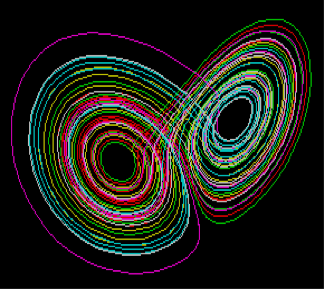
Figure 1: The Lorenz Attractor
However, what does appear to pass as a crucial feature of chaos for Batterman—a definition if you will—is the presence of a kind of “stretching and folding” mechanism in the dynamics (see the discussion on p. 49 and figure 5 of his essay). Basically such a mechanism will cause some trajectories to converge rapidly while causing other trajectories to diverge rapidly. Such a mechanism would tend to cause trajectories issuing from various points in some small neighborhood of state space to mix and separate in rather dramatic ways. For instance, some initially neighboring trajectories on the Lorenz attractor (Figure 1) become separated, where some end up on one wing while others end up on the other wing. This stretching and folding is part of what leads to definitions of the distance between trajectories in state space as increasing (diverging) on average.
The presence of such a mechanism in the dynamics, Batterman believes, is a necessary condition for chaos. As such, this defining characteristic could be applied to both mathematical models and real-world systems, though the identification of such mechanisms in target systems may be rather tricky.
1.2.5 Quantitative Definitions of Chaos
Let us start with the property of SDIC and distinguish weak and strong forms of sensitive dependence (somewhat following Smith 1998). Weak sensitive dependence can be characterized as follows. Consider the propagator, J(x(t)), a function that evolves trajectories x(t) in time (an example of a propagator is given in the Appendix). Let x(0) and y(0) be initial conditions for two different trajectories. Then,
(WSD)
A system characterized by J(x(t)) has the property of weak sensitive dependence on its initial conditions if and only if ∃ε>0 ∀x(0) ∀δ>0 ∃t>0 ∃y(0) [ |x(0) − y(0)| < δ and |J(x(t)) − J(y(t))| > ε ].
The essential idea is that the propagator acts so that no matter how close together x(0) and y(0) are the trajectory initiating from y(0) will eventually diverge by ε from the trajectory initiating from x(0). However, WSD does not specify the rate of divergence (it is compatible with linear rates of divergence) nor does it specify how many points surrounding x(0) will give rise to diverging trajectories (it could be a set of any measure, e.g., zero). Typically, a system is not considered chaotic unless nearly all points in state space are capable of giving rise to diverging trajectories.
On the other hand, chaos is usually characterized by a strong form of sensitive dependence:
(SD)
∃λ such that for almost all points x(0), ∀δ>0 ∃t>0 such that for almost all points y(0) in a small neighborhood (δ) around x(0) [ |x(0) − y(0)|<δ and |J(x(t)) − J(y(t))| ≈ |J(x(0)) − J(y(0))|eλt ],
where the “almost all” caveat is understood as applying for all points in state space except a set of measure zero. Here, λ is interpreted as the largest global Lyapunov exponent (see the Appendix) and is taken to represent the average rate of divergence of neighboring trajectories issuing forth from some small neighborhood centered around x(0). Exponential growth is implied if λ>0 (convergence if λ<0). In general, such growth cannot go on forever. If the system is bounded in space and in momentum, there will be limits as to how far nearby trajectories can diverge from one another.
Note that according to SD, Poincaré's first two examples would fail to qualify as characterizing a chaotic system (the first one exhibits an entire range of growth rates from zero to larger than exponential, while the second one exhibits growth larger than exponential). On the other hand, these examples do satisfy WSD.
One strategy for devising a definition for chaos is to begin with discrete maps and then generalize to the continuous case. For example, if one begins with a continuous system, by using a Poincaré surface of section—roughly, a two-dimensional plane is defined and one plots the intersections of trajectories with this plane—a discrete map can be generated. If the original continuous system exhibits chaotic behavior, then the discrete map generated by the surface of section with also be chaotic because the surface of section will have the same topological properties as the continuous system. Robert Devaney's influential definition of chaos (1989) was proposed in this fashion.
Let f be a function defined on some state space S. In the continuous case, f would vary continuously on S and we might have a differential equation specifying how f varies. In the discrete case, f can be thought of as a mapping that can be iterated or reapplied a number of times. To indicate this, we can write f n(x), meaning f is applied iteratively n times. For instance, f 3(x) would indicate f has been applied three times, thus f 3(x) = f(f(f(x))) (Robert May's 1976 review article has a nice discussion of this for the logistic map, xn + 1 = rxn(1 − xn), which arises in modeling the dynamics of predator-prey relations, for instance.). Furthermore, let K be a subset of S. Then f(K) represents f applied to the set of points K, that is, f maps the set K into f(K). If f(K) = K, then K is an invariant set under f.
Now Devaney's definition of chaos can be stated as follows:
(Chaosd)
A continuous map f is chaotic if f has an invariant set K⊆S such that
- f satisfies WSD on K,
- The set of points initiating periodic orbits are dense in K, and
- f is topologically transitive on K.
Topological transitivity is the following notion: consider open sets U and V around the points u and v respectively. Regardless how small U and V are, some trajectory initiating from U eventually visits V. This condition roughly guarantees that trajectories starting from points in U will eventually fill S densely. Taken together, these three conditions represent an attempt to precisely characterize the kind of irregular, aperiodic behavior we expect chaotic systems to exhibit.
Devaney's definition has the virtues of being precise and compact. However, objections have been raised against it. Since the time he proposed his definition, it has been shown that (2) and (3) imply (1) if the set K has an infinite number of elements (see Banks et al. 1992), although this result does not hold for sets with finite elements. More to the point, the definition seems counterintuitive in that it emphasizes periodic orbits rather than aperiodicity, but the latter seems a much better characterization of chaos. After all, it is precisely the lack of periodicity that is characteristic of chaos. To be fair to Devany, however, he casts his definition in terms of unstable periodic points, the kind of points where trajectories issuing forth from neighboring points would exhibit WSD. If the set of unstable periodic points is dense in K, then we have a guarantee that the kinds of aperiodic orbits characteristic of chaos will be abundant. Some have argued that (2) is not even necessary for characterizing chaos (e.g., Robinson 1995, pp. 83–4). Furthermore, nothing in Devaney's definition hints at the stretching and folding of trajectories, which appears to be a necessary condition for chaos from a qualitative perspective. Peter Smith (1998, pp. 176–7) suggests that Chaosd is, perhaps, a consequence rather than a mark of chaos.
Another possibility for capturing the concept of the folding and stretching of trajectories so characteristic of chaotic dynamics is the following:
(Chaosh)
A discrete map f is chaotic if, for some iteration n ≥1, it maps the unit interval I into a horseshoe (see Figure 2).
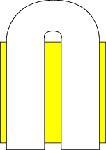
Figure 2: The Smale Horseshoe
To construct the Smale horseshoe map (Figure 2), start with the unit square (indicated in yellow). First, stretch it in the y direction by more than a factor of two. Then compress it in the x direction by more than a factor of two. Now, fold the resulting rectangle and lay it back onto the square so that the construction overlaps and leaves the middle and vertical edges of the initial unit square uncovered. Repeating these stretching and folding operations leads to the Samale attractor.
This definition has at least two virtues. First, it can be proven that Chaosh implies Chaosd. Second, it yields exponential divergence, so we get SD, which is what many people expect for chaotic systems. However, it has a significant disadvantage in that it cannot be applied to invertible maps, the kinds of maps characteristic of many systems exhibiting Hamiltonian chaos. A Hamiltonian system is one where the total kinetic energy plus potential energy is conserved; in contrast, dissipative systems lose energy through some dissipative mechanism such as friction or viscosity. Hamiltonian chaos, then, is chaotic behavior in a Hamiltonian system.
Other possibile definitions have been suggested in the literature. For example (Smith 1998, pp. 181–2),
(Chaoste)
A discrete map is chaotic just in case it exhibits topological entropy: Let f be a discrete map and {Wi} be a partition of a bounded region W containing a probability measure which is invariant under f. Then the topological entropy of f is defined as hT(f) = sup{Wi}h(f,{Wi}), where sup is the supremum of the set {Wi}.
Roughly, given the points in a neighborhood N around x(0) less than ε away from each other, after n iterates of f the trajectories initiating from the points in N will differ by ε or greater, where more and more trajectories will differ by at least ε as n increases. In the case of one-dimensional maps, however, it can be shown that Chaosh implies Chaoste. So this does not look to be a basic definition, though it is often more useful for proving theorems relative to the other definitions.
Another candidate, often found in the physics literature, is
(Chaosλ)
A discrete map is chaotic if it has a positive global Lyapunov exponent.
The meaning of positivity here is that a global Lyapunov exponent is positive for almost all points in the specified set S. This definition certainly is directly connected to SD and is one physicists often use to characterize systems as chaotic. Furthermore, it offers practical advantages when it comes to calculations and can often be “straightforwardly” related to experimental data in the sense of examining data sets generated from physical systems for global Lyapunov exponents.[2]
1.2.6 Trouble with Lyapunov Exponents and Sensitive Dependence
One might think that SD, Chaoste or Chaosλ could be sufficient for defining chaos, but these characterizations run into problems from simple counterexamples. For instance, consider a discrete dynamical system with S = [0, ∞), the absolute value as a metric (i.e., as the function that defines the distance between two points) on R, and a mapping f : [0, ∞) → [0,∞), f(x) = cx, where c>1. In this dynamical system, all neighboring trajectories diverge exponentially fast, but all accelerate off to infinity. However, chaotic dynamics is usually characterized as being confined to some attractor—a strange attractor (see sec. 5.1 below) in the case of dissipative systems, the energy surface in the case of Hamiltonian systems. This confinement need not be due to physical walls of some container. If, in the case of Hamiltonian chaos, the dynamics is confined to an energy surface (by the action of a force like gravity), this surface could be spatially unbounded. So at the very least some additional conditions are needed (e.g., that guarantee trajectories in state space are dense).
In much physics and philosophy literature, something like the following set of conditions seems to be assumed as adequately defining chaos:
- Trajectories are confined due to some kind of stretching and folding mechanism.
- Some trajectory orbits are aperiodic, meaning that they do not repeat themselves on any time scales.
- Trajectories exhibit SD or Chaosλ.
Of these three features, (c) is often taken to be crucial to defining SDIC and is often suspected as being related to the other two. That is to say, exponential growth in the separation of neighboring trajectories characterized by λ is taken to be a property of a particular kind of dynamics that can only exist in nonlinear systems and models.
Though the favored approaches to defining chaos involve global Lyapunov exponents, there are problems with this way of defining SDIC (and, hence, characterizing chaos). First, the definition of global Lyapunov exponents involves the infinite time limit (see the appendix), so, strictly speaking, λ only characterizes growth in uncertainties as t increases without bounds, not for any finite t. So the combination ∃λ and ∃t>0 in SD is inconsistent. At best, SD can only hold for the large time limit and this implies that chaos as a phenomenon can only arise in this limit, contrary to what we take to be our best evidence. Furthermore, neither our models nor physical systems run for infinite time, but an infinitely long time is required to verify the presumed exponential divergence of trajectories issuing from infinitesimally close points in state space.
On might try to get around these problems by invoking the standard physicist's assumption that an infinite-time limit can be used to effectively represent some large but finite elapsed time. However, one reason to doubt this assumption in the context of chaos is that the calculation of finite-time Lyapunov exponents do not usually lead to on-average exponential growth as characterized by global Lyapunov exponents (e.g., Smith, Ziehmann and Fraedrich 1999). In general, for finite times the propagator varies from point to point in state space (i.e., it is a function of the position x(t) in state space and only approaches a constant in the infinite time limit), implying that the local finite-time Lyapunov exponents vary from point to point. Therefore, trajectories diverge and converge from each other at various rates as they evolve in time—the uncertainty does not vary uniformly in the chaotic region of state space (Smith, Ziehmann and Fraedrich 1999; Smith 2000). This is in contrast to global Lyapunov exponents which are on-average global measures of trajectory divergence and which imply that uncertainty grows uniformly (for λ>0), but such uniform growth rarely occurs outside a few simple mathematical models. For instance, the Lorenz, Moore-Spiegel, Rössler, Henon and Ikeda attractors all possess regions dominated by decreasing uncertainties in time, where uncertainties associated with different trajectories issuing forth from some small neighborhood shrink for the amount of time trajectories remain within such regions (e.g., Smith, Ziehmann and Fraedrich 1999, pp. 2870–9; Ziehmann, Smith and Kurths 2000, pp. 273–83). Hence, on-average exponential growth in trajectory divergence is not guaranteed for chaotic dynamics. Linear stability analysis can indicate when nonlinearities can be expected to dominate the dynamics, and local finite-time Lyapunov exponents can indicate regions on an attractor where these nonlinearities will cause all uncertainties to decrease—cause trajectories to converge rather than diverge—so long as trajectories remain in those regions.
To summarize, the folklore that trajectories issuing forth from neighboring points will diverge on-average exponentially in a chaotic region of state space is false in any sense other than for infinitesimal uncertainties in the infinite time limit.
The second problem with the standard account is that there simply is no implication that finite uncertainties will exhibit an on-average growth rate characterized by any Lyapunov exponents, local or global. For example, the linearized dynamics used to derive global Lyapunov exponents presupposes infinitesimal uncertainties (appendix (A1)–(A5)). But when uncertainties are finite, such dynamics do not apply and no valid conclusions can be drawn about the dynamics of finite uncertainties from the dynamics of infinitesimal uncertainties. Certainly infinitesimal uncertainties never become finite in finite time—barring super exponential growth. Even if infinitesimal uncertainties became finite after a finite time, that would presuppose the dynamics is unconfined, whereas the interesting features of nonlinear dynamics usually take place in subregions of state space. Presupposing an unconfined dynamics would be inconsistent with the features we are typically trying to capture.
Can the on average exponential growth rate characterizing SD ever be attributed legitimately to diverging trajectories if their separation is no longer infinitesimal? Examining simple models (e.g., the Baker's transformation) might seem to indicate yes. However, answering this question requires some care for more complex systems like the Lorenz or Moore-Spiegel attractors. It may turn out that the rate of divergence in the finite separation between two nearby trajectories in a chaotic region changes character numerous times over the course of their winding around in state space, sometimes faster, sometimes slower than that calculated from global Lyapunov exponents, sometimes contracting, sometimes diverging (Smith, Ziehmann and Fraedrich 1999; Ziehmann, Smith and Kurths 2000). But in the long run, some of these trajectories could effectively diverge as if there was on-average exponential growth in uncertainties as characterized by global Lyapunov exponents. However, it is conjectured that the set of initial points in the state space exhibiting this behavior is a set of measure zero, meaning, in this context, that although there are an infinite number of points exhibiting this behavior, this set represents zero percent of the number of points composing the attractor. The details of the kinds of divergence (convergence) neighboring trajectories undergo turn on the detailed structure of the dynamics (i.e., it is determined point-by-point by local growth and convergence of finite uncertainties and not by any Lyapunov exponents).
But as a practical matter, all finite uncertainties saturate at the diameter of the attractor. This is to say, that the uncertainty reaches some maximum amount of spreading after a finite time and is not well quantified by global measures derived from Lyapunov exponents (e.g., Lorenz 1965). So the folklore—that on-average exponential divergence of trajectories characterizes chaotic dynamics—is misleading for nonlinear models and systems, in particular the ones we want to label as chaotic. Therefore, drawing an inference from the presence of positive global Lyapunov exponents to the existence of on-average exponentially diverging trajectories is invalid. This has implications for defining chaos because exponential growth parametrized by global Lyapunov exponents turn out to not be an appropriate measure. Hence, SD or Chaosλ turn out to be misleading definitions of chaos.
Finally, I want to briefly draw attention to the observer-dependent nature of global Lyapunov exponents in the special theory of relativity. As has been recently demonstrated (Zheng, Misra and Atmanspacher 2003), global Lyapunov exponents change in magnitude under Lorentz transformations, though not in sign—e.g., positive Lyapunov exponents are always positive under Lorentz transformations. Moreover, under Rindler transformations, global Lyapunov exponents are not invariant so that a system characterized as chaotic under SD or Chaosλ for an accelerated Rindler observer turns out to be nonchaotic for an inertial Minkowski observer and any system that is chaotic for a an inertial Minkowski observer is nonchaotic for an accelerated Rindler observer. So along with the simultaneity problems raised for observers by Einstein's theory of special relativity (see the entry on conventionality of simultaneity), chaos, at least under SD or Chaosλ, turns out to also have observer-dependent features for pairs of observers in different reference frames. What these features mean for our understanding of the phenomenon of chaos are largely unexplored.
1.2.7 Taking Stock
There is no consensus regarding a precise definition of chaotic behavior among mathematicians and physicists, although physicists often prefer Chaosh or Chaosλ. The latter definitions, however, are trivially false for finite uncertainties in real systems and of limited applicability for mathematical models. It also appears to be the case that there is no one “right” or “correct” definition, but that varying definitions have varying strengths and weaknesses regarding tradeoffs on generality, theorem-generation, calculation ease and so forth. The best candidates for necessary conditions for chaos still appear to be (1) WSD, which is rather weak, or (2) the presence of stretching and folding mechanisms (“pulls trajectories apart” in one dimension while “compressing them” in another).
The other worry is that the definitions we have been considering may only hold for our mathematical models, but may not be applicable to target systems. The formal definitions seek to fully characterize chaotic behavior in mathematical models, but we are also interested in capturing chaotic behavior in physical and biological systems as well. Phenomenologically, the kinds of chaotic behavior we see in real-world systems exhibit features such as SDIC, aperiodicity, unpredictability, instability under small perturbations and apparent randomness. However, given that target systems run for only a finite amount of time and that the uncertainties are always larger than infinitesimal, such systems violate the assumptions necessary for deriving SD. In other words, even if we have good statistical measures that yield on average exponential growth in uncertainties for a physical data set, what guarantee do we have that this corresponds with the exponential growth of SD? After all, any growth in uncertainties (alternatively, any growth in distance between neighboring trajectories) can be fitted with an exponential. If there is no physical significance to global Lyapunov exponents (because they only apply to infinitesimal uncertainties), then one is free to choose any parameter to fit an exponential for the growth in uncertainties.
So where does this leave us regarding a definition of chaos? Are all our attempts at definitions inadequate? Is there only one definition for chaos, and if so, is it only a mathematical property or also a physical one? Do we, perhaps, need multiple definitions (some of which are nonequivalent) to adequately characterize such complex and intricate behavior? Is it reasonable to expect that the phenomenological features of chaos of interest to physicists and applied mathematicians can be captured in precise mathematical definitions given that there may be irreducible vagueness in the characterization of these features? From a physical point of view, isn't a phenomenological characterization sufficient for the purpose of identifying and exploring the underlying mechanisms responsible for the stretching and folding of trajectories? The answers to these questions largely lie in our purposes for the kinds of inquiry in which we are engaged (e.g., proving rigorous mathematical theorems vs. detecting chaotic behavior in physical data vs. designing systems to control such behavior).
2. What is Chaos “Theory”?
One often finds references in the literature to “chaos theory”. For instance, Kellert characterizes chaos theory as “the qualitative study of unstable aperiodic behavior in deterministic nonlinear systems” (Kellert 1993, p. 2). In what sense is chaos a theory? Is it a theory in the same sense that electrodynamics or quantum mechanics are theories?
Answering such questions is difficult if for no other reason than that there is no consensus about what a theory is. Options here range from the axiomatic or syntactic view of the logical positivists and empiricists (see Vienna Circle) to the semantic or model-theoretic view (see models in science), to Kuhnian (see Thomas Kuhn) and less rigorous conceptions of theories. The axiomatic view of theories appears to be inapplicable to chaos. There are no axioms—no laws—no deductive structures, no linking of observational statements to theoretical statements whatsoever in the literature on chaotic dynamics.
Kellert's (1993) focus on chaos models is suggestive of the semantic view of theories, and many texts and articles on chaos focus on models (e.g., logistic map, Henon map, Lorenz attractor). Briefly, on the semantic view, a theory is characterized by (1) some set of models and (2) the hypotheses linking these models with idealized physical systems. The mathematical models discussed in the literature are concrete and fairly well understood, but what about the hypotheses linking chaos models with idealized physical systems? In the chaos literature, there is a great deal of discussion of various robust or universal patterns and the kinds of predictions that can and cannot be made using chaotic models. Moreover, there is a lot of emphasis on qualitative predictions, geometric “mechanisms” and patterns, but this all comes up short of spelling out hypotheses linking chaos models with idealized physical systems.
One possibility is to look for hypotheses about how such models are deployed when studying real physical systems. Chaos models seem to be deployed to ascertain various kinds of information about bifurcation points, period doubling sequences, the onset of chaotic dynamics, strange attractors and other denizens of the chaos zoo of behaviors. The hypotheses connecting chaos models to physical systems would have to be filled in if we are to employ the semantic conception fully. I take it these would be hypotheses about, for example, how strange attractors reconstructed from physical data relate to the physical system from which the data were originally recorded, or about how a one-dimensional map for a particular full nonlinear model (idealized physical system) was developed using, say, Poincaré surface of section techniques.
Such an approach does seem consistent with the semantic view as illustrated with classical mechanics. There we have various models such as the harmonic oscillator and hypotheses about how these models apply to idealized physical systems, including specifications of spring constants and their identification with mathematical terms in a model, small oscillation limits, etc. But in classical mechanics there is a clear association between the models of a theory and the state spaces definable over the variables of those models, with a further hypothesis about the relationship between the model state space and that of the physical system being modeled (the faithful model assumption, §1.2.3). One can translate between the state spaces and the models and, in the case of classical mechanics, can read the laws off as well (e.g., Newton's laws of motion are encoded in the possibilities allowed in the state spaces of classical mechanics).
Unfortunately, the connection between state spaces, chaotic models and laws is less clear. Indeed, there are no good candidates for laws of chaos over and above the laws of classical mechanics, and some, like Kellert, explicitly deny that chaos modeling is getting at laws at all (1993, ch. 4). Furthermore, the relationship between the state spaces of chaotic models and the spaces of idealized physical systems is quite delicate, which seems to be a dissimilarity between classical mechanics and “chaos theory”. In the former case, we can translate between models and state spaces. In the latter, we can derive a state space for chaotic models from the full nonlinear model, but we cannot reverse the process and get back to the nonlinear model state space from that of the chaotic model. One might expect the hypotheses connecting chaos models with idealized physical systems to piggy back on the hypotheses connecting classical mechanics models with their corresponding idealized physical systems. But it is neither clear how this would work in the case of nonlinear systems in classical mechanics, nor how this would work for chaotic models in biology, economics and other disciplines.[3]
Additionally, there is another potential problem that arises from thinking about the faithful model assumption, namely what is the relationship or mapping between model and target system? Is it one-to-one as we standardly assume? Or is it a one-to-many relation (several different nonlinear models of the same target system or, potentially, vice versa) or a many-to-many relationship? For many classical mechanics problems—namely, where linear models or force functions are used in Newton's second law—the mapping or translation between model and target system appears to be straightforwardly one-to-one. However, in nonlinear contexts, where one might be constructing a model from a data set generated by observing a system, there are potentially many nonlinear models that can be constructed, where each model is as empirically adequate to the system behavior as any other. Is there really only one unique model for each target system and we simply do not know which is the “true” one (say, because of underdeterminiation problems—see scientific realism)? Or is there really no one-to-one relationship between our mathematical models and target systems?
Moreover, an important feature of the semantic view is that models are only intended to capture the crucial features of physical systems and always involve various forms of abstraction and idealization (see models in science). These caveats are potentially deadly in the context of nonlinear dynamics. Any errors in our models for such systems, no matter how accurate our initial data, will lead to errors in predicting real systems as these errors will grow (perhaps rapidly) with time. This brings out one of the problems with the faithful model assumption that is hidden, so to speak, in the context of linear systems. In the latter context, models can be erroneous by leaving out “negligible” factors and, at least for reasonable times, our model predictions do not differ significantly with the physical systems we are modeling (wait long enough, however, and such predictions will differ significantly). In nonlinear contexts, by contrast, there are no “negligible” factors as even the smallest omission in a nonlinear model can lead to disastrous effects because the differences these terms would have made versus their absence potentially can be rapidly amplified as the model evolves (see §3).
Another possibility is to drop hypotheses connecting models with target systems and simply focus on the defining models of the semantic view of theories. This is very much the spirit of the mathematical theory of dynamical systems. There the focus is on models and their relations, but there is no emphasis on hypotheses connecting these models with physical systems, idealized or otherwise. Unfortunately, this would mean that chaos theory would be only a mathematical theory and not a physical one.
Both the syntactic and semantic views of theories focus on the formal structure of theoretical bodies, and their “fit” with theorizing about chaotic dynamics seem quite problematic. In contrast, perhaps one should conceive of chaos theory in a more informal way, say along the lines of Kuhn's (1996) analysis of scientific paradigms. There is no emphasis on the precise structure of scientific theories in Kuhn's picture of science. Rather, theories are cohesive, systematic bodies of knowledge defined mainly by the roles they play in normal science practice within a dominant paradigm. There is a very strong sense in literature about chaos that a “new paradigm” has emerged out of chaos research with its emphasis on unstable rather than stable behavior, on dynamical patterns rather than on mechanisms, on universal features (e.g., Feigenbaum's number) rather than laws, and on qualitative understanding rather than on precise prediction. Whether or not chaotic dynamics represents a genuine scientific paradigm, the use of the term ‘chaos theory’ in much of the scientific and philosophical literature has the definite flavor of characterizing and understanding complex behavior rather than an emphasis on the formal structure of principles and hypotheses.
3. Nonlinear Models, Faithfulness and Confirmation
Given a target system to be modeled, and invoking the faithful model assumption, there are two basic approaches to model confirmation discussed in the philosophical literature on modeling following a strategy known as piecemeal improvement (I will ignore bootstrapping approaches as they suffer similar problems, but only complicate the discussion). These piecemeal strategies are also found in the work of scientists modeling real-world systems and represent competing approaches vying for government funding (for an early discussion, see Thompson 1957).
The first basic approach is to focus on successive refinements to the accuracy of the initial data used by the model while keeping the model itself fixed (e.g., Laymon 1989, p. 359). The idea here is that if a model is faithful in reproducing the behavior of the target system to some degree, refining the precision of the initial data fed to the model will lead to its behavior monotonically converging to the target system's behavior. This is to say that as the uncertainty in the initial data is reduced, a faithful model's behavior is expected to converge to the target system's behavior. The import of the faithful model assumption is that if one were to plot the trajectory of the target system in an appropriate state space, the model trajectory in the same state space would monotonically become more like the system trajectory on some measure as the data is refined (I will ignore difficulties regarding appropriate measures for discerning similarity in trajectories; see Smith 2000).
The second basic approach is to focus on successive refinements of the model while keeping the initial data fixed (e.g., Wimsatt 1987). The idea here is that if a model is faithful in reproducing the behavior of the target system, refining the model will produce an even better fit with the target system's behavior. This is to say that if a model is faithful, successive improvements will lead to its behavior monotonically converging to the target system's behavior. Again, the import of the faithful model assumption is that if one were to plot the trajectory of the target system in an appropriate state space, the model trajectory in the same state space would monotonically become more like the system trajectory as the model is made more realistic.
What both of these basic approaches have in common is that piecemeal monotonic convergence of model behavior to target system behavior is a mark for confirmation of the model (Koperski 1998). By either improving the quality of the initial data or improving the quality of the model, the model in question reproduces the target system's behavior monotonically better and yields predictions of the future states of the target system that show monotonically less deviation with respect to the behavior of the target system. In this sense, monotonic convergence to the behavior of the target system is a key criterion for whether the model is confirmed. If monotonic convergence to the target system behavior is not found by pursuing either of these basic approaches, then the model is considered to be disconfirmed.
For linear models it is easy to see the intuitive appeal of such piecemeal strategies. After all, for linear systems of equations a small change in the magnitude of a variable is guaranteed to yield a proportional change in the output of the model. So by making piecemeal refinements to the initial data or to the linear model only proportional changes in model output are expected. If the linear model is faithful, then making small improvements “in the right direction” in either the initial data or the model itself can be tracked by improved model performance. The qualifier “in the right direction”, drawing upon the faithful model assumption, means that the data quality really is increased or that the model really is more realistic (captures more features of the target system in an increasingly accurate way), and is signified by the model's monotonically improved performance with respect to the target system.
However, both of these basic approaches to confirming models encounter serious difficulties when applied to nonlinear models, where the principle of linear superposition no longer holds. In the first approach, successive small refinements in the initial data used by nonlinear models is not guaranteed to lead to any convergence between model behavior and target system behavior. Any small refinements in initial data can lead to non-proportional changes in model behavior rendering this piecemeal convergence strategy ineffective as a means for confirming the model. A refinement of the quality of the data “in the right direction” is not guaranteed to lead to a nonlinear model monotonically improving in capturing the target system's behavior. The small refinement in data quality may very well lead to the model behavior diverging away from the system's behavior.[4]
In the second approach, keeping the data fixed but making successive refinements in nonlinear models is also not guaranteed to lead to any convergence between model behavior and target system behavior. With the loss of linear superposition, any small changes in the model can lead to non-proportional changes in model behavior again rendering the convergence strategy ineffective as a means for confirming the model. Even if a small refinement to the model is made “in the right direction”, there is no guarantee that the nonlinear model will monotonically improve in capturing the target system's behavior. The small refinement in the model may very well lead to the model behavior diverging away from the system's behavior.
So whereas for linear models piecemeal strategies might be expected to lead to better confirmed models (presuming the target system exhibits only stable linear behavior), no such expectation is justified for nonlinear models deployed in the characterization of nonlinear target systems. Even for a faithful nonlinear model, the smallest changes in either the initial data or the model itself may result in non-proportional changes in model output, an output that is not guaranteed to “move in the right direction” even if the small changes are made “in the right direction” (of course, this lack of guarantee of monotonic improvement also raises questions about what “in the right direction” means, but I will ignore these difficulties here).
Intuitively, piecemeal convergence strategies look to be dependent on the perfect model scenario. Given a perfect model, refining the quality of the data should lead to monotonic convergence of the model behavior to the target system's behavior, but even this expectation is not always justifiable for perfect models (cf. Judd and Smith 2001; Smith 2003). On the other hand, given good data, perfecting a model intuitively should also lead to monotonic convergence of the model behavior to the target system's behavior. By making small changes to a nonlinear model, hopefully based on improved understanding of relevant features of the target system (e.g., the physics of weather systems or the structures of economies), there is no guarantee that such changes will produce monotonic improvement in the model's performance with respect to the target system's behavior. The loss of linear superposition, then, leads to a similar lack of guarantee of a continuous path of improvement as the lack of guarantee of piecemeal confirmation. And without such a guaranteed path of improvement, there is no guarantee that a faithful nonlinear model can be perfected.
Of course, we do not have perfect models. But even if we did, they are unlikely to live up to our intuitions about them (Judd and Smith 2001; Judd and Smith 2004). If there is either no perfect model for a target system, or the perfect model still does not guarantee monotonic improvement with respect to the target system's behavior, the traditional piecemeal confirmation strategies will fail. Merely faithful nonlinear models are not guaranteed to converge to nonlinear target system behavior under piecemeal confirmation strategies.
The bottom line for modeling nonlinear systems, then, is that piecemeal monotonic convergence of nonlinear models to target system behavior is not guaranteed. This is the upshot of the failure of the principle of linear superposition. No matter how faithful the model, no guarantee can be made of piecemeal monotonic improvement of a nonlinear model's behavior with respect to the target system (of course, if one waits for long enough times piecemeal confirmation strategies will also fail for linear systems). Furthermore, problems with these confirmation strategies will arise whether one is seeking to model point-valued trajectories in state space or one is using probability densities defined on state space.
One possible response to the piecemeal confirmation problems discussed here is to turn to a Bayesian framework for confirmation, but similar problems arise here for nonlinear models. Given that there are no perfect models in the model class to which we would apply a Bayesian scheme and given the fact that imperfect models will fail to reproduce or predict target system behavior over time scales that may be short compared to our interests, there again is no guarantee that monotonic improvement can be achieved for our nonlinear models (I leave aside the problem that having no perfect model in our model class renders many Bayesian confirmation schemes ill-defined).
For nonlinear models, faithfulness can fail and perfectibility cannot be guaranteed, raising questions about scientific modeling practices and our understanding of them. However, the implications of the loss of linear superposition reach father than this. Policy assessment often utilizes model forecasts and if the models and systems lying at the core of policy deliberations are nonlinear (e.g., the climate or economy), then policy assessment will be affected by the same lack of guarantee as model confirmation. Suppose administrators are using a nonlinear model in the formulation of economic policies designed to keep GDP ever increasing while minimizing unemployment (among achieving other socio-economic goals). While it is true that there will be some uncertainty generated by running the model several times over slightly different data sets and parameter settings, assume that policies taking these uncertainties into account to some degree can be fashioned. Once in place, the policies need assessment regarding their effectiveness and potential adverse effects, but such assessment will not involve merely looking at monthly or quarterly reports on GDP and employment data to see if targets are being met. The nonlinear economic model driving the policy decisions will need to be rerun to check if trends are indeed moving “in the right direction” with respect to the earlier forecasts. But, of course, data for the model have now changed and there is no guarantee that the model will produce a forecast with this new data that fits well with the old forecasts used to craft the original policies. Nor is there a guarantee of any fit between the new runs of the nonlinear model and the economic data being gathered as part of ongoing monitoring of the economic policies. How, then, are policy makers to make reliable assessments of policies? The same problem—that small changes in data or model in nonlinear contexts are not guaranteed to yield proportionate model outputs or monotonically improved model performance—also plagues policy assessment using nonlinear models. Such problems are largely unexplored.
4. Chaos, Determinism and Quantum Mechanics
One of the exciting features of SDIC is that there is no lower limit on just how small some change or perturbation can be—the smallest of effects will eventually be amplified up affecting the behavior of any system exhibiting SDIC. A number of authors have argued that chaos through SDIC opens a door for quantum mechanics to “infect” chaotic classical mechanics systems (e.g., Hobbs 1991; Barone et al. 1993; Kellert 1993; Bishop and Kronz 1999; Bishop forthcoming). The essential point is that the nature of particular kinds of nonlinear dynamics—those which exhibit stretching and folding (confinement) of trajectories, where there are no trajectory crossings, and which exhibit aperiodic orbits—apparently open the door for quantum effects to change the behavior of chaotic macroscopic systems. The central argument runs as follows and is known as the sensitive dependence argument (SD argument for short):
- For systems exhibiting SDIC, trajectories starting out in a highly localized region of state space will diverge on-average exponentially fast from one another.
- Quantum mechanics limits the precision with which physical systems can be specified to a neighborhood in phase space of no less than (2π ⁄ h)N, where h is Plank's constant (with units of action) and N is the dimension of the system in question.
- Given enough time and the quantum mechanical bound on the neighborhood ε for the initial conditions, two trajectories of the same chaotic system will have future states localizable to a much larger region δ in phase space (from (A) and (B)).
- Therefore, quantum mechanics will influence the outcomes of chaotic systems leading to a violation of unique evolution.
Premise (A) makes clear that SD is the operative definition for characterizing chaotic behavior in this argument, invoking exponential growth characterized by the largest global Lyapunov exponent. Premise (B) expresses the precision limit for the state of minimum uncertainty for measuring momentum and position pairs in an N-dimensional quantum system (note, the exponent is 2N in the case of measuring uncorrelated electrons).[5] The conclusion of the argument in the form given here is actually stronger than that quantum mechanics can influence a macroscopic system exhibiting SDIC, but also that determinism fails for such systems because of such influences. Briefly, the reasoning runs as follows. Because of SDIC, nonlinear chaotic systems whose initial states can be located only within a small neighborhood ε of state space will have future states that can be located only within a much larger patch δ. For example, two isomorphic nonlinear systems of classical mechanics exhibiting SDIC, whose initial states are localized within ε, will have future states that can be localized only within δ. Since quantum mechanics sets a lower bound on the size of the patch of initial conditions, unique evolution must fail for nonlinear chaotic systems.
The SD argument does not go through as smoothly as some of its advocates have thought, however. There are difficult issues regarding the appropriate version of quantum mechanics (e.g., von Neumann, Bohmian or decoherence theories; see entries under quantum mechanics), the nature of quantum measurement theory (collapse vs. non-collapse theories; see measurement in quantum theory), and the selection of the initial state characterizing the system that must be resolved before one can say clearly whether or not unique evolution is violated (Bishop forthcoming). For instance, just because quantum effects might influence macroscopic chaotic systems doesn't guarantee that determinism fails for such systems. Whether quantum interactions with nonlinear macroscopic systems exhibiting SDIC contribute indeterministically to the outcomes of such systems depends on the currently undecidable question of indeterminism in quantum mechanics and the measurement problem.
There is a serious open question as to whether the indeterminism in quantum mechanics is simply the result of ignorance due to epistemic limitations or if it is an ontological feature of the quantum world. Suppose that quantum mechanics is ultimately deterministic, but that there is some additional factor, a hidden variable as it is often called, such that if this variable were available to us, our description of quantum systems would be fully deterministic. Another possibility is that there is an interaction with the broader environment that accounts for how the probabilities in quantum mechanics arise (physicists call this approach “decoherence”). Under either of these possibilities, we would interpret the indeterminism observed in quantum mechanics as an expression of our ignorance, and, hence, indeterminism would not be a fundamental feature of the quantum domain. It would be merely epistemic in nature due to our lack of knowledge or access to quantum systems. So if the indeterminism in QM is not ontologically genuine, then whatever contribution quantum effects make to macroscopic systems exhibiting SDIC would not violate unique evolution. In contrast, suppose it is the case that quantum mechanics is genuinely indeterministic; that is, all the relevant factors of quantum systems do not fully determine their behavior at any given moment. Then the possibility exists that not all physical systems traditionally thought to be in the domain of classical mechanics can be described using strictly deterministic models, leading to the need to approach the modeling of such nonlinear systems differently (e.g., Bishop and Kronz 1999, pp. 138–9).
Moreover, the possible constraints of nonlinear classical mechanics systems on the amplification of quantum effects must be considered on a case-by-case basis. For instance, damping due to friction can place constraints on how quickly amplification of quantum effects can take place before they are completely washed out (Bishop forthcoming). And one has to investigate the local finite-time dynamics for each system because these may not yield any on-average growth in uncertainties (e.g., Smith, Ziehmann, Fraedrich 1999).
In summary, there is no abstract, a priori reasoning establishing the truth of an SD argument; the argument can only be demonstrated on a case-by-case basis. Perhaps detailed examination of several cases would enable us to make some generalizations about how wide spread the possibilities for the amplification of quantum effects are.
5. Questions about Realism and Explanation
Two traditional topics in philosophy of science are realism and explanation. Although not well explored in the context of chaos, there are plenty of interesting questions regarding both topics deserving of further exploration.
5.1 Realism and Chaos
Chaos raises a number of questions about scientific realism (see scientific realism) only some of which will be touched on here. First and foremost, scientific realism is usually formulated as a thesis about the status of unobservable terms in scientific theories and their relationship to entities, events and processes in the real world. In other words, theories make various claims about features of the world and these claims are approximately true. But as we saw in §2, there are serious questions about formulating a theory of chaos, let alone determining how this theory fares under scientific realism. It seems more reasonable, then, to discuss some less ambitious realist questions regarding chaos: Is chaos a real phenomenon? Do the various denizens of chaos, like fractals, actually exist?
This leads us back to the faithful model assumption (§1.2.3). Recall this assumption maintains that our model equations faithfully capture target system behavior and that the model state space faithfully represents the actual possibilities of the target system. Is the sense of faithfulness here that of actual correspondence between mathematical models and features of actual systems? Or can faithfulness be understood in terms of empirical adequacy alone, a primarily instrumentalist construal of faithfulness? Is a realist construal of faithfulness threatened by the mapping between models and systems potentially being one-to-many or many-to-many?
A related question is whether or not our mathematical models are simulating target systems or merely mimicking their behavior. To be simulating a system suggests that there is some actual correspondence between the model and the target system it is designed to capture. On the other hand, if a mathematical model is merely mimicking the behavior of a target system, there is no guarantee that the model has any genuine correspondence to the actual qualities of the target system. The model merely imitates behavior. These issues become crucial for modern techniques of building nonlinear dynamical models from large time series data sets (e.g., Smith 1992), for example the sunspot record or the daily closing value of a particular stock for some specific period of time. In such cases, after performing some tests on the data set, the modeler sets to work constructing a mathematical model that reproduces the time series as its output. Do such models only mimic behavior of target systems? Where does realism come into the picture?
A further question regarding chaos and realism is the following: Is chaos only a feature of our mathematical models or is it a genuine feature of actual systems in our world? This question is well illustrated by a peculiar geometric structure of dissipative chaotic models called a strange attractor, which can form based upon the stretching and folding of trajectories in state space. Strange attractors normally only occupy a subregion of state space, but once a trajectory wanders close enough to the attractor, it is caught near the surface of the attractor for the rest of its future.
One of the characteristic features of strange attractors is that they posses self-similar structure. If we were to magnify any small portion of the attractor, we would find that the magnified portion would look identical to the regular-sized region. If we were to magnify the magnified region, we would see the identical structure repeated again. Continuous repetition of this process would yield the same results. The self-similar structure is repeated on arbitrarily small scales. An important geometric implication of self-similarity is that there is no inherent size scale so that we can take as large a magnification of as small a region of the attractor as we want and a statistically similarly structure will be repeated (Hilborn 1994, p. 56). In other words strange attractors for chaotic models have an infinite number of layers of repetitive structure. This type of structure allows trajectories to remain within a bounded region of state space by folding and intertwining with one another without ever intersecting or repeating themselves exactly.
Strange attractors also are often characterized as possess noninteger or fractal dimension (though not all strange attractors have such dimensionality). The type of dimensionality we usually meet in physics as well as in everyday experience is characterized by integers. A point has dimension zero; a line has dimension one; a square has dimension two; a cube has dimension three and so on. As a generalization of our intuitions regarding dimensionality, consider a large square. Suppose we fill this large square with smaller squares each having an edge length of ε. The number of small squares needed to completely fill the space inside the large square is N(ε). Now repeat this process of filling the large square with small squares, but each time let the length ε get smaller and smaller. In the limit as ε approached zero, we would find that the ratio ln N(ε) ⁄ ln(1 ⁄ ε) equals two just as we would expect for a 2-dimensional square. You can imagine the same exercise of filling a large 3-dimensional cube (a room, say) with smaller cubes and in the limit of ε approaching zero, we would arrive at a dimension of three.
When we apply this generalization of dimensionality to the geometric structure of strange attractors, we find that we get noninteger results. Roughly this means that if we try to apply the same procedure of “filling” the structure formed by the strange attractor with small squares or cubes, in the limit as ε approaches zero the result is noninteger. Whether one is examining a set of nonlinear mathematical equations or analyzing the time series data from an experiment, the presence of self-similarity or noninteger dimension are indications that the chaotic behavior of the system under study is dissipative (nonconservative) rather than Hamiltonian (conservative).
Although there is no universally accepted definition for strange attractors or fractal dimension among mathematicians, the more serious question is whether strange attractors and fractal dimensions are properties of our models only or also of real-world systems. For instance, empirical investigations of a number of real-world systems indicate that there is no infinitely repeating self-similar structure like that of strange attractors (Avnir, et al. 1998; see also Shenker 1994). At most, one finds self-similar structure repeated on two or three spatial scales in the reconstructed state space and that is it. This appears to be more like a prefractal, where self-similar structure exists on only a finite number of length scales. That is to say, prefractals repeat their structure under magnification only a finite number of times rather than infinitely as in the case of a fractal. So this seems to indicate that there are no genuine strange attractors with fractal dimension in real systems, but possibly only attractors having prefractal geometries with self-similarity on a limited number of spatial scales.
On the other hand, the dissipative chaotic models used to characterize some real-world systems all exhibit strange attractors with fractal geometries. So it looks like fractal geometries in chaotic model state spaces bear no relationship to the pre-fractal features of real-world systems. In other words, these fractal features of many of our models are clearly false of the target systems though the models themselves may still be useful in helping scientists locate interesting dynamics of target systems characterized by prefractal properties. Scientific realism and usefulness look to part ways here. At least many of the strange attractors of our models play the role of useful fictions.
There are two caveats to this line of thinking, however. First, the prefractal character of the analyzed data sets (e.g. by Avnir, et al. 1998) could be an artifact of the way data is massaged before it is analyzed or due to the analog-to-digital conversion that must take place before data analysis can begin. Reducing real number valued data to sixteen bits would destroy fractal structure. If so, the infinitely self-similar structures of fractals in our models might not be such a bad approximation after all.
A different reason, though, to suspect that physical systems cannot have such self-repeating structures “all the way down” is that at some point the classical world gives way to the quantum world, where things change so drastically that there cannot be a strange attractor because the state space changes. Hence, we are applying a model carrying a tremendous amount of excess, fictitious structure to understand features of physical systems. This looks like a problem because one of the key structures playing a crucial role in chaos explanations—the infinitely intricate structure of the strange attractor—would then be absent from the corresponding physical system.
According to Peter Smith (1998, ch. 3), one might be justified in employing obviously false chaos models because the infinitely intricate structure of strange attractors (1) is the result of relatively simple stretching and folding mechanisms and (2) many of the points in state space of interest are invariant under this stretching and folding mechanism. These features represent kinds of simplicity that can be had at the (perhaps exorbitant!) cost of fictitious infinite structure. The strange attractor exhibits this structure and the attractor is a sign of some stretching and folding process. The infinite structure is merely geometric extra baggage, but the robust properties like period-doubling sequences, onset of chaos, and so forth are real enough. This has the definite flavor of being antirealist about some key elements of explanation in chaos (§5.2) and has been criticized as such (Koperski 2001).
Instead of trying to squeeze chaos into scientific realism's mold, then, perhaps it is better to turn to an alternative account of realism, structural realism (e.g., Worrall 1994). Roughly, the idea is that realism in scientific practices hinges on the structural relations of phenomena. So structural realism tends to focus on the causal structures in well-confirmed scientific hypotheses and theories. The kinds of universal structural features identified in chaotic phenomena in realms as diverse as physics, biology and economics is very suggestive of some form of structural realism and, indeed, look to play key roles in chaos explanations (see below). Though, again, there are significant worries that infinitely repeating self-similar structure might not be realized in physical systems. On a structural approach to realism regarding chaos models, one faces the difficulty that strange attractors are at best too gross an approximation to structure of physical attractors and at worst terribly misleading.
Perhaps other kinds of geometric structures associated with chaos would qualify on a structural realist view. After all, it also seems to be the case that realism for chaos models has more to do with processes—namely stretching and folding mechanisms at work in target systems. But here the connection with realism and chaos models would come indirectly via an appeal to the causal processes at work in the full nonlinear models taken to represent physical systems. Perhaps the fractal character of strange attractors is an artifact introduced through the various idealizations and approximations used to derive such chaotic models. If so, then perhaps there is another way to arrive at more realistic chaos models that have prefractal attractors.
5.2 The Nature of Chaos Explanations
Chaos has been invoked as an explanation for, or as contributing substantially to explanations of, real-world behaviors. Some examples are epileptic seizures, heart fibrillation, neural processes, chemical reactions, weather, industrial control processes and even forms of message encryption. Aside from irregular behavior of real-world systems, chaos is also invoked to explain features like the actual trajectories exhibited in a given state space or the sojourn times of trajectories in particular regions of state space. But what, exactly, is the role chaos plays in these various explanations? More succinctly, what are chaos explanations?
The nature of scientific explanation (see the entry on scientific explanation) in the literature on chaos is thoroughly under-discussed to put it mildly. Traditional accounts for scientific explanation like covering-law, causal mechanical and unification models all present various kinds of drawbacks when applied to chaotic phenomena. For instance, if there are no laws lying at the heart of chaos explanations—and it does not seem credible that laws could really play a role in such explanations—covering-law models do not look promising as candidates for chaos explanations.
Roughly speaking, the causal-mechanical model of explanation maintains that science provides understanding of diverse facts and events by showing how these fit into the causal structure of the world. If chaos is a behavior exhibited by nonlinear systems (mathematical and physical), then it seems reasonable to think that there might be some mechanisms or processes standing behind this behavior. After all, chaos is typically understood to be a property of the dynamics of such systems, and dynamics is usually determined by the processes at work and their interactions. The links between causal mechanisms and behaviors in the causal-mechanical model are supposed to be reliable links, along the lines of if mechanism C is present, behavior B typically follows. In this sense, chaos explanations, understood on the causal-mechanical model, are envisioned as providing reliable connections between mechanisms and the chaotic behavior exhibited by systems containing such mechanisms.
On the other hand, the basic idea of unification accounts of explanation is that science provides understanding of diverse facts and events by showing how these may be unified by a much smaller set of factors (e.g., laws or causes; in the case of the latter, one might consider this a species of causal explanation). Perhaps one can argue that chaos is a domain or set of a limited number of patterns and tools for explaining/understanding a set of characteristic behaviors found in diverse phenomena spread across physics, chemistry, biology, economics, social psychology, and so forth. In this sense the set of patterns or structures (e.g., “stretching and folding”) might make up the explanatory store unifying our understanding of all the diverse phenomena behaving chaotically.
5.2.1 Explanation, Faithful Models and Chaos
Both causal and unification accounts, as typically conceived, assume that theories are in place and that the models of those theories play some role in explanation. In causal accounts, causal processes are key components of the models. In unification accounts, laws might be the ultimate explanatory factors, but we often connect laws with physical systems via models. To be explanatory, however, such accounts must make the faithful model assumption; namely, that our models (and their state spaces) are faithful in what they say about the world.
Recall that SD—exponential divergence of neighboring trajectories—is taken by many to be a necessary condition for chaos. As we saw in §3, it would be difficult if not impossible to confirm when we have a model serving as a good explanation because, for instance, the slightest refinement of initial conditions can lead to wildly differing behavior. So on many standard approaches to confirmation and models, it would be difficult to say when we had a good explanation. Even if we push the faithful model assumption to its extreme limit—i.e., assuming the model is perfect—we run into tricky questions regarding confirmation since there are too many states indistinguishable from the actual state of the system yielding empirically indistinguishable trajectories in the model state space (Judd and Smith 2001).
Perhaps with chaos explanation we should either search for a process yielding the “stretching and folding” in the dynamics (causal form of explanation) or we should search for the common properties such behavior exhibits (unification form of explanation) underlying the behavior of the nonlinear systems of interest. In other words, we want to be able to understand why systems exhibit SDIC, aperiodicity, randomness, and so forth. But these are the properties characterizing chaotic behavior, so the unification account of explanation sounds like it may ultimately involve appealing to the properties in need of explanation.
The explanatory picture becomes more complicated by shifting away from SD as characterized by a positive global Lyapunov exponent and settling for what may be more realistic, namely the effects of divergence/contraction characterized by finite-time Lyapunov exponents. However, even in this case, it appears that the properties to which one appeals on a unification account pick out the patterns of chaos that we want to understand: how do these properties arise? It seems that unification accounts are still at a disadvantage in characterizing chaos explanations.
Suppose we appealed to strange attractors in our models or in state space reconstruction techniques. Would this be evidence that there is a strange attractor in the target system's behavior? Modulo worries raised in §5.1, even if the presence of a strange attractor in the state space was both a necessary and sufficient condition for the model being chaotic, this would not amount to an explanation of chaotic behavior in the target system. First, the strange attractor is an object in state space, which is not the same as saying that the actual system behaves as if there is a strange attractor in the physical space of its activity. A trajectory in a state space is a way of gaining useful information about the target system (via the faithful model assumption), but it is different from trajectories developed by looking at how a system's properties change with respect to time. Just because a trajectory of a system in state space is spiraling ever closer to the strange attractor does not imply that the target system's behavior in physical space is somehow approaching that attractor (except possibly under the perfect model scenario). Second, but related, the presence of a strange attractor would only be a mark of chaos, not an explanation for why chaotic properties are being exhibited by a system. It seems we still need to appeal to processes and interactions causing the dynamics to have the characteristic properties we associate with chaos.
At this point, a question implied at the end of the previous subsection arises, namely what is effecting the unification in chaos explanations? Unification models of explanation typically posit an explanatory store of a relatively small number of laws or mechanisms that serve to explain or unify a diverse set of phenomena. A standard example is that of Newtonian mechanics providing a small set of principles that could serve to explain phenomena as diverse as projectile motions, falling bodies, tides, planetary orbits and pendula. In this way, we say that Newtonian mechanics unified a diverse set of phenomena by showing that they all were governed by a small set of physical principles. Now, if a unification construal of chaos explanations only focuses on the mathematical similarities in behaviors of diverse phenomena (e.g., period doubling route to chaos or SDIC), then one can legitimately question whether the relevant sense of unification is in play in chaos explanations. The “explanatory store” of chaos explanations is indeed a small set of mathematical and geometrical features, but is this the wrong store (compare with the physical principles of Newtonian mechanics)? However, if unification is supposed to be achieved through underlying mechanisms producing these mathematical and geometrical features, then the explanatory store appears to be very large and heterogeneous—the mechanisms in physics are different from those in biology, are different from those in ecology, are different from those in economics are different from those in social psychology…Once again, the causal-mechanical model appears to make more sense for characterizing the nature of chaos explanations.
5.2.2 Chaos and Understanding
If this were all there was to the story of chaos explanations, then a causal account of explanation looks more promising. But it would also be the case that there is nothing special about such explanations: there are processes and interactions that cause the dynamics to have chaotic properties. But Stephen Kellert (1993, ch. 4) maintains that there is something new about chaotic dynamics, forcing us to rethink explanation when it comes to chaos models. His proposal for chaos explanations as yielding qualitative understanding of system behavior suggests that causal accounts, at least, do not fit well with what is going on in chaos research.
Kellert first focuses on one of the key intuitions driving many views in debates on scientific explanation: namely, that science provides understanding or insight into phenomena. Chaos explanations, according to Kellert, achieve understanding by constructing, elaborating and applying simple dynamical models. He gives three points of contrast between this approach to understanding and what he takes to be the standard approach to understanding in the sciences. The first is that chaos explanations involve models that are holistic rather than microreductionist. Models of the latter type seek to break systems down into their constituent parts and look for law-like relations among the parts. In contrast, many of the mathematical tools of chaotic dynamics are holistic in that they extract or reveal information about the behavior of the model system as a whole not readily apparent from the nonlinear equations of the model themselves. Methods like state space reconstruction and sections-of-surface can reveal information implicit in the nonlinear equations. Developing one- and two-dimensional maps from the model equations can also provide this kind of information directly, and are much simpler than the full model equations.
Whereas the first point of contrast is drawn from the practice of physics, the second is logical. After reducing the system to its parts, the next step in the standard approach to understanding, according to Kellert, is to construct a “deductive scheme, which yields a rigorous proof of the necessity (or expectability) of the situation at hand” (1993, p. 91). What makes this logical is the emphasis on “deductive scheme.” The approach in chaotic dynamics makes no use of deductive inferences. Specifically, instead of looking at basic principles, propositions, etc., and making deductive inferences, chaos explanations appeal to computer simulations because of the difficulty or even impossibility of deducing the chaotic behavior of the system from the model equations (e.g., no proof of SD for the Lorenz model based on the governing equations).
The third point of contrast is historical. In contexts where linear superposition holds, a full specification of the instantaneous state plus the equations of motion yield all the information about the system there is to know (e.g., pendulum and projectile motion). Although a full specification of such states is impossible, very small errors in specifying such states lead to very small deviations between model and target system behaviors, at least for short times and good models. By contrast, in nonlinear contexts, where linear superposition fails, a full specification of an instantaneous state of the system plus the equations of motion does not yield all the information there is about the system, e.g., if there are memory effects (hysteresis). Then we also need to know the history of the system as well (whether it started out below the critical point or above the critical point, say). So chaos explanations must also take model histories into account.
What kind of understanding is achieved in chaos explanations? Kellert argues we get (1) predictions of qualitative behavior rather than quantitative detail, (2) geometric mechanisms rather than causal processes, and (3) patterns rather than law-like necessity.
Regarding (1), detailed predictions regarding individual trajectories fail rather rapidly for chaotic models when there is any error in specification of the initial state. So, says Kellert, instead we predict global behaviors of models and have an account of limited predictability in chaotic models. But many of these behaviors can be precisely predicted (e.g., control parameter values[6] at which various bifurcations occur, the onset of chaos, the return of n-periodic orbits). (1) amounts to important, but limited insight. On this view we are able to predict when to expect qualitative features of the nonlinear dynamics to undergo a sudden change, but chaos models do not yield precise values of system variables. We get the latter values by running full-blow computer simulations on the full nonlinear model equations, provided the degrees of freedom are reasonable. In this sense chaos explanations are complimentary to the full model simulation because the former can tell us when/where to expect dynamical changes like the onset of complicated dynamics in the latter.
Regarding (2), chaos explanation is not a species of causal explanation. That is to say, chaos explanations do not focus on or reveal processes and interactions giving rise to the dynamics; rather, they reveal large-scale geometric features of the dynamics. Kellert argues the kinds of mechanisms on which chaos explanations focus are not causal, but geometric. Part of the reason why he puts things this way is that he views typical causal accounts of explanation as operating in a reductive mode: trace the individual causal processes and their interactions to understand the behavior of the system. But chaos explanations, according to Kellert, eschew this detailed level, focusing instead on the behavior of systems as wholes. Indeed, chaos explanations tend to group models and systems together as exhibiting similar patterns of behavior without regard for their underlying causal differences. Causal processes are ignored; instead, universal patterns of behavior are the focus. And it is the qualitative information about the geometric features of the model that are key to chaos explanations for Kellert.
Regarding (3), if scientific understanding is only to be achieved via appeal to universal laws expressing nomic necessity—still a strong intuition among many philosophers—then chaos explanations definitely do not measure up. Chaos explanations do not rely on nomic considerations at all; rather, they rely on patterns of behavior and various properties characterizing this behavior. In brief, chaos studies search for patterns rather than laws.
But suppose we change the notion of laws from universal statements of nomic necessity to phenomenological regularities (e.g., Cartwright 1983, 1999; Dupré 1993)? Could chaos explanations then be understood as a search for such phenomenological laws at the level of wholes? After all, chaos as a field is not proposing any revisions to physical laws the way relativity and quantum mechanics did. Rather, if it is proposing anything, it is new levels of analysis and techniques for this analysis. Perhaps it is at the level of wholes that interesting phenomenological regularities exist that cannot be probed by microreductionist approaches. But this feature, at least on first blush, may not count against the microreductionist in anything other than an epistemological sense, that is, holistic methodologies are more effective for answering some questions chaos raises.
This dynamical understanding, as Kellert denotes it, achieved by chaos models would suggest that typical causal accounts of explanation are aimed at a different level of understanding. In other words, causal accounts look much more consonant with studying the full nonlinear model. Chaos explanation, by contrast, pursues understanding by using reduced equations derived from various techniques, though still often loosely based on the full nonlinear equations. This way of viewing things suggests that there is a kind of unification going on in chaos explanation after all. A set of behavior patterns serves as the explanatory or unificatory features bringing together the appearance of similar features across a very diverse set of phenomena and disciplines (note: Kellert does not discuss unification accounts). This, in turn, suggests a further possibility: a causal account of explanation is more appropriate at the level of the full model, while a unification account perhaps is more appropriate at the level of the chaotic model. The approaches would be complementary rather than competing.
Furthermore, the claim is that study of such chaotic models can give us understanding of the behavior in corresponding real-world systems. Not because the model trajectories are isomorphic to the system trajectories; rather, because there is a topological or geometric similarity or correspondence between the models and the systems being modeled. This is a different version of the faithful model assumption in that now the topological/geometric features of target systems are taken to be faithfully represented by our chaotic models.
5.2.3 Nothing New under the Sun?
In contrast to Kellert, Peter Smith makes it clear that he thinks there is nothing particularly special about chaos explanations in comparison with explanation in mathematical physics in general (1998, ch. 7). Perhaps it simply is the case that mathematical physics explanations are not well captured by philosophical accounts of explanation and this mismatch—peculiarly highlighted in a sexy field such as chaos—could provide some of the reason for why people have taken chaos explanations to pose radical challenges to traditional philosophical accounts of explanation.
In particular, Smith takes issue with Kellert's view that chaos explanations are, in the main, qualitative rather than quantitative. He points out that we can calculate Lyapunov exponents, bifurcation points as control parameters change, and even use chaos models be predict the values of evolving dynamical variables—“individual trajectory picture”—at least for some short time horizon. So perhaps there is more quantitative information to be gleaned from chaos models than Kellert lets on (this is particularly true if we turn to statistical methods of prediction). Furthermore, Smith argues that standard physics explanations, along with quantitative results, always emphasize the qualitative features of models as well.
We might agree, then, that there is nothing particularly special or challenging about chaos explanations relative to other kinds of explanation in physics regarding qualitative/quantitative understanding. What does seem to be the case is that chaos models—and nonlinear dynamics models generally—make the extraction of usefulness quantitative information more difficult. What is exhibited by methodological approaches in chaos is not that different from what happens in other areas of mathematical physics, where the mathematics is intractable and the physical insight is short. Moreover, there is no guarantee that in the future we will not make some kind of breakthrough placing chaos models on a much sounder first principles footing, so there does not seem to be much substance to the claim that chaos explanations are different in kind from other modes of explanation in mathematical physics.
5.3 Taking Stock
Kellert's discussion of “dynamic understanding” and Peter Smith's critical remarks both overlap in their agreement that various robust or universal features of chaos are important for chaos studies The idea of focusing on universal features such as patterns, critical numbers, and so forth suggests that some form of unification account of explanation is what is at work in chaos explanations: group together all examples of chaotic behavior via universal patterns and other features (e.g., period doubling sequences). There is disagreement on the extent to which the methodologies of current chaos research present any radically new challenges to the project of scientific explanation.
Even if there is not something radically new here regarding scientific explanation, the kind of understanding provided by chaos models is still challenging to clarify. One problem is that this “dynamic understanding” appears to be descriptive only. That is, Kellert seems to be saying we understand how chaos arises when we can point to a period doubling sequence or to the presence of a strange attractor for instance. But this appears to be only providing distinguishing marks for chaos rather than yielding genuine insight into what lies behind the behavior, i.e., the cause of the behavior. Kellert eschews causes regarding chaos explanations and there is a fairly straightforward reason for this: the simplified models of chaos appear to be just mathematics (e.g., one dimensional maps) loosely based on the original nonlinear equations. In other words, it looks as if the causes have been squeezed out! So the question of whether causal, unificationist or some other approach to scientific explanation best captures chaos research remains open.
Moreover, since all these simplified models use roughly the same mathematics, why should we think it is surprising that we see the same patterns arise over and over again in disparate models? After all, if all the traces of processes and interactions—the causes—have been removed from chaos models, as Kellert suggests, why should it be surprising that chaos models in physics, biology, economics and social psychology exhibit similar behavior? If it really boils down to the same mathematics in all the models, then what is it we are actually coming to understand by using these models?
6. Some Broader Implications of Chaos
There have been some discussions regarding the wider implications of chaos for other domains of philosophical inquiry. Two of the more thought-provoking ones will be surveyed here.
6.1 Free Will and Consciousness
A number of authors have looked to quantum mechanics to help explain consciousness and free will (e.g., Compton 1935; Eccles 1970; Penrose 1991, 1994 and 1997; Beck and Eccles 1992; Stapp 1993; Kane 1996). Still it has been less clear to many that quantum mechanics is relevant to consciousness and free will. For example, an early objection to quantum effects influencing human volitions was offered by philosopher J. J. C. Smart (1963, pp. 123–4).[7] Even if indeterminism was true at the quantum level, Smart argued that the brain remains deterministic in its operations because quantum events are insignificant by comparison. After all a single neuron is known to be excited by on the order of a thousand molecules, each molecule consisting of ten to twenty atoms. Quantum effects though substantial when focusing on single atoms are presumed negligible when focusing on systems involving large numbers of molecules. So it looks like quantum effects would be too insignificant in comparison to the effects of thousands of molecules to play any possible role in consciousness or deliberation.
Arguments such as Smart's do not take into consideration the possibility for amplifying quantum effects through the interplay between SDIC at the level of the macroscopic world on the one hand and quantum effects on the other (see §4). SD arguments purport to demonstrate that chaos in classical systems can amplify quantum fluctuations due to sensitivity to the smallest changes in initial conditions. Along these lines suppose (somewhat simplistically) the patterns of neural firings in the brain correspond to decision states. The idea is that chaos could amplify quantum events causing a single neuron to fire that would not have fired otherwise. If the brain (a macroscopic object) is also in a chaotic dynamical state, making it sensitive to small disturbances, this additional neural firing, small as it is, would then be further amplified to the point where the brain states would evolve differently than if the neuron had not fired. In turn these altered neural firings and brain states would carry forward such quantum effects affecting the outcomes of human choices.
There are several objections to this line of argument. First, the presence of chaos in the brain and its operations is an empirical matter that is hotly debated (Freeman and Skarda 1987; Freeman 1991, 2000; Kaneko, Tsuda and Ikegami 1994 pp. 103–189; Vandervert 1997; Diesmann, Gewaltig and Aertsen 1999; Lehnertz 2000). It should be pointed out, however, that these discussions typically assume SD or Chaosλ as the definition of chaos. Perhaps all that is really needed for sensitivity to and amplification of quantum effects in the brain is the loss of principle of superposition found in nonlinear systems. Second, these kinds of sensitivity arguments depend crucially on how quantum mechanics itself and measurements are interpreted as well as the status of indeterminism (§4). Third, although in the abstract sensitivity arguments seem to lead to the conclusion that the smallest of effects can be amplified, applying such arguments to concrete physical systems shows that the amplification process may be severely constrained. In the case of the brain, we currently do no know what constraints on amplification exist.
An alternative possibility avoiding many of the difficulties exhibited in the chaos+quantum mechanics approach is suggested by the research on far-from-equilibrium systems by Ilya Prigogine and his Brussels-Austin Group (Bishop 2004). Their work purports to offer reasons to search for a different type of indeterminism at both the micro and macrophysical levels.
Consider a system of particles. If the particles are distributed uniformly in position in a region of space, the system is said to be in thermodynamic equilibrium (e.g., cream uniformly distributed throughout a cup of coffee). In contrast, if the system is far-from-equilibrium (nonequilibrium) the particles are arranged so that highly ordered structures might appear (e.g., a cube of ice floating in tea). The following properties characterize nonequilibrium statistical systems: large number of particles, high degree of structure and order, collective behavior, irreversibility, and emergent properties. The brain possesses all these properties, so that the brain can be considered a nonequilibrium system (an equilibrium brain is a dead brain!).
Let me quickly sketch a simplified version of the approach to point out why the developments of the Brussels-Austin Group offer an alternative for investigating the connections between physics, consciousness and free will. Conventional approaches in physics describe systems using particle trajectories as a fundamental explanatory element of their models, meaning that the behavior of a model is derivable from the trajectories of the particles composing the model. The equations governing the motion of these particles are reversible with respect to time (they can be run backwards and forwards like a film). When there are too many particles involved to make these types of calculations feasible (as in gases or liquids), coarse-grained averaging procedures are used to develop a statistical picture of how the system behaves rather than focusing on the behavior of individual particles.
In contrast the Brussels-Austin approach views nonequilibrium systems in terms of nonlinear models whose fundamental explanatory elements are distributions; that is to say, the arrangements of the particles are the fundamental explanatory elements and not the individual particles and trajectories.[8] The equations governing the behavior of these distributions are generally irreversible with respect to time. In addition focusing exclusively on distribution functions opens the possibility that macroscopic nonequilibrium models are irreducibly indeterministic, an indeterminism that has nothing to do with ignorance about the system. If so, this would mean probabilities are as much an ontologically fundamental element of the macroscopic world as they are of the microscopic and are free of the interpretive difficulties found in conventional quantum mechanics.
One important insight of the Brussels-Austin Group's shift away from trajectories to distributions as fundamental elements is that explanation also shifts from a local context (set of particle trajectories) to a global context (distribution of the entire set of particles). Systems acting as a whole may produce collective effects that are not reducible to a summation of the trajectories and subelements composing the system (Bishop 2004 and 2008). The brain exhibits this type of collective behavior in many circumstances (Engel, et al. 1997) and the work of Prigogine and his colleagues gives us another tool for trying to understand that behavior. Moreover, nonlinear nonequilibrium models also exhibit SDIC, so there are a number of possibilities in such approaches for very rich dynamical description of brain operations and cognitive phenomena (e.g., Juarrero 1999). Though the Brussels-Austin approach to nonequilibrium statistical mechanics is still speculative and contains some open technical questions (Bishop 2004), it offers an alternative for exploring the relationship between physics, consciousness and free will as well as pointing to a new possible source for indeterminism to be explored in free will theories.
Whether approaches applying chaotic dynamics to understanding the nature of consciousness and free will represent genuine advances remain an open question. For example, if the world is deterministic, then the invocation of SDIC in cognitive dynamics (e.g., Kane 1996) may provide a sophisticated framework for exploring deliberative processes, but would not be sufficient for incompatibilist notions of freedom. On the other hand, if indeterminism (quantum mechanical or otherwise) is operative in the brain, the challenge still remains for indeterminists like Robert Kane (1996) to demonstrate that agents can effectively harness such indeterminism by utilizing the exquisite sensitivity provided by nonlinear dynamics to ground and explain free will. Questions about realism and explanation in chaotic dynamics (§5) are relevant here as well as the faithful model assumption.
6.2 Human and Divine Action in a Nonlinear World
There has also been much recent work applying the perspective of dynamical systems to cognition and action, drawing explicitly on such properties as attractors, bifurcations, SDIC and other denizens of the nonlinear zoo (e.g., van Gelder 1995; Kelso 1995; Port and van Gelder 1995; Juarrero 1999; Tsuda 2001). The basic idea is to deploy the framework of nonlinear dynamics for interpreting neural and cognitive activity as well as complex behavior. It is then hoped that patterns of neural, cognitive and human activity can be explained as the results of nonlinear dynamical processes involving causal interactions and constraints at multiple levels (e.g., neurons, brains, bodies, physical environments). Such approaches are highly suggestive, but also face challenges. For instance, as mentioned in the previous section, the nature of neural and cognitive dynamics is still much disputed. Ultimately, it is an empirical matter whether these dynamics are largely nonlinear or not. Moreover, the explanatory power of dynamical systems approaches relative to rival computational approaches has been challenged (e.g., Clark 1998). Again, questions about realism and explanation in chaotic dynamics (§5) are relevant here as well as the faithful model assumption.
Furthermore, John Polkinghorne (among others) has proposed interpreting the randomness in macroscopic chaotic models and systems as representing a genuine indeterminism rather than merely a measure of our ignorance (1991, pp. 34–48). The idea is that such openness or indeterminism is not only important to the free will and action we experience (pp. 40–1), but also for divine action in the world (e.g., Polkinghorne 1988 and 1989). In essence the sensitivity to small changes exhibited by the systems and models studied in chaotic dynamics, complexity theory and nonequilibrium statistical mechanics is taken to represent an ontological opening in the physical order for divine activity. However the sensitivity upon which Polkinghorne relies would also be open to quantum influences whether deterministic or indeterministic. Furthermore, as mentioned previously in connection with the Brussels-Austin program, much rides on whether a source for indeterminism in chaotic behavior can be found. If Polkinghorne's suggestion amounts to simply viewing the world as if chaos harbors indeterminism, then it seems there is no room ontologically for any divine action in Polkinghorne's and similar approaches.
7. Conclusion
Chaos and nonlinear dynamics are not only rich areas for scientific investigation, but also raise a number of interesting philosophical questions. The majority of these questions, however, remain thoroughly under studied by philosophers.
Appendix: Global Lyapunov Exponents
Bibliography
- Aristotle (1985) [OTH], On the Heavens,; in. J. Barnes (ed.), The Complete Works of Aristotle: The Revised Oxford Translation, Vol 1. Princeton: Princeton University Press.
- Avnir, D., Biham, O., Lidar, D. and Malcai, O. (1998), “Is the Geometry of Nature Fractal?” Science, 279: 39–40.
- Banks, J., Brooks, J. Cairns, G. Davis, G. and Stacey, P. (1992), “On Devaney's Definition of Chaos”, American Mathematical Monthly, 99: 332–334.
- Barone, S. R., Kunhardt, E. E., Bentson, J. and Syljuasen (1993), “Newtonian Chaos + Heisenberg Uncertainty = Macroscopic Indeterminacy”, American Journal Of Physics, 61: 423–7.
- Batterman, R. W. (1993), “Defining Chaos”, Philosophy of Science, 60: 43–66.
- Beck, F. and Eccles, J. (1992), “Quantum Aspects of Brain Activity and the Role of Consciousness”, in Proceedings of the National Academy of Science (United States), 89: 11357–11361.
- Berkovitz, J, Frigg, R. and Kronz, F. (2006), “The Ergodic Hierarchy, Randomness and Chaos”, Studies in History and Philosophy of Modern Physics, 37: 661–691.
- Bishop, R. C. (2002a), “Chaos, Indeterminism, and Free Will”, in R. Kane (ed.), The Oxford Handbook of Free Will. Oxford: Oxford University Press, pp. 111–124.
- Bishop, R. C. (2002b), “Deterministic and Indeterministic Descriptions”, in H. Atmanspacher and R. Bishop (eds.), Between Chance and Choice: Interdisciplinary Perspectives on Determinism. Thorverton: Imprint Academic, pp. 5–31.
- Bishop, R. C. (2003), “On Separating Prediction from Determinism”, Erkenntnis, 58: 169–188.
- Bishop, R. C. (2004), “Nonequilibrium Statistical Mechanics Brussels-Austin Style”, Studies in History and Philosophy of Modern Physics, 35: 1–30.
- Bishop, R. C. (2005), “Anvil or Onion? Determinism as a Layered Concept”, Erkenntnis, 63: 55–71.
- Bishop, R. C. (2006), “Determinism and Indeterminism”, in D. M. Borchert (ed. in chief), Encyclopedia of Philosophy, Second Edition. Farmington Hills, MI: Macmillian Reference, Vol. 3, pp. 29–35.
- Bishop, R. C. (2008), “Downward Causation in Fluid Convection,”, Synthese 160: 229-248.
- Bishop, R. C. (forthcoming), “What Could Be Worse than the Butterfly Effect?”, Canadian Journal of Philosophy.
- Bishop, R. C. and Kronz, F. K. (1999), “Is Chaos Indeterministic?” in M. L. Dalla Chiara, R. Guintini and F. Laudisa (eds.) Language, Quantum, Music: Selected Contributed Papers of the Tenth International Congress of Logic, Methodology & Philosophy of Science, Florence, August, 1995. Dordrecht, The Netherlands: Kluwer Academic Publishers, pp. 129–141.
- Cartwright, N. (1983), How the Laws of Physics Lie. Oxford: Clarendon Press.
- Cartwright, N. (1999), The Dappled World: A study of the Boundaries of Science. Cambridge: Cambridge University Press.
- Clark, A. (1998), “Time and Mind”, Journal of Philosophy, 95: 354–376.
- Compton, A.(1935), The Freedom of Man. New Haven: Yale University Press.
- Diesmann M., Gewaltig M-O., Aertsen A. (1999), “Stable Propagation of Synchronous Spiking in Cortical Neural Networks”, Nature, 402: 529–533.
- Devaney, R. (1989), “Dynamics of Simple Maps”, Proceedings of Symposia in Applied Mathematics, 39: 1–24.
- Duhem, P. (1982), The Aim and Structure of Physical Theory. Princeton: Princeton University Press.
- Dupré, J. (1993), The Disorder of Things: Metaphysical Foundations of the Disunity of Science. Cambridge, MA: Harvard University Press.
- Eccles, J. (1970), Facing Reality. New York: Springer.
- Engel, A., Roelfsema, P., König, P. and Singer, W. (1997), “Neurophysiological Relevance of Time”, in H. Atmanspacher and E. Ruhnau (eds.), Time, Temporality, Now: Experiencing Time and Concepts of Time in an Interdisciplinary Perspective. Berlin: Springer, pp. 133–157.
- Ford, J. and Mantica, G. (1992), “Does Quantum Mechanics Obey the Correspondence Principle? Is It Complete?” American Journal of Physics, 60: 1086–1097.
- Fox, R. F. (1990), “Chaos, Molecular Fluctuations, and the Correspondence Limit”, Physical Review A, 41: 2969–2976.
- Freeman, W. J. (1991), “Nonlinear Dynamics in Olfactory Information Processing”, in J. Davis and H. Eichenbaum (eds.) Olfaction. Cambridge, MA: MIT Press.
- Freeman, W. J. (2000), How Brains Make Up Their Minds. New York: Columbia University Press.
- Freeman, W. J. and Skarda, C. A. (1987), “How Brains Make Chaos in Order to Make Sense of the World”, Behavioral and Brain Sciences, 10: 161–195.
- van Gelder, T. (1995), “What Might Cognition Be if not Computation?”, Journal of Philosophy, 92: 345–381.
- Gutzwiller, M. C. (1992), “Quantum Chaos”, Scientific American, 266 (January): 78–84.
- Hadamard, J. [1922] (1952), Lectures on Cauchy's Problem in Linear Partial Differential Equations, New York: Dover.
- Hilborn, R. C. (1994), Chaos and Nonlinear Dynamics: An Introduction for Scientists and Engineers, Oxford: Oxford University Press.
- Hobbs, J. (1991), “Chaos and Indeterminism”, Canadian Journal of Philosophy, 21: 141–164.
- Hunt, B. R. and Yorke, J. A. (1993), “Maxwell on Chaos”, Nonlinear Science Today, 3(1): 1–4.
- Jensen, R. V. (1987), “Classical Chaos”, American Scientist, 75 (March-April): 168–181.
- Jensen, R. V. (1992), “Quantum Chaos”, Nature, 355: 311–318.
- Jones, R. (1990), “Determinism in Deterministic Chaos”, in A. Fine, M Forbes, and L. Wessels (eds.) PSA 1990, Volume 2, East Lansing: Philosophy of Science Association, pp. 537–549.
- Juarrero, A. (1999), Dynamics in Action: Intentional Behavior as a Complex System, Cambridge, MA: MIT Press.
- Judd, K., and Smith, L. (2001), “Indistinguishable States I: Perfect Model Scenario”, Physica D 151: 125–141.
- Judd, K., and Smith, L. (2004), “Indistinguishable States II: Imperfect Model Scenarios”, Physica D 196: 224–242.
- Kane, R. (1996), The Significance of Free Will, Oxford: Oxford University Press.
- Kaneko, K. and Tsuda, I. (2000), Complex Systems: Chaos and Beyond, Berlin: Springer.
- Kaneko, K., Tsuda, I. and Ikegami, T. (eds.), (1994), “Constructive Complexity and Artificial Reality: Proceedings of the Oji International Seminar on Complex Systems—from Complex Dynamical Systems to Sciences of Artificial Reality”, Physica D 75: 1–448.
- Kellert, S. (1993), In the Wake of Chaos, Chicago University Press.
- King, C. C. (1995), “Fractal Neurodynamics and Quantum Chaos: Resolving the Mind-Brain Paradox Through Novel Biophysics”, in E. MacCormack, E. and M.I. Stamenov, M.I. (eds.) Fractals of Brain, Fractals of Mind. Amsterdam and Philadelphia: John Benjamins.
- Koperski, J. (1998), “Models, Confirmation and Chaos”, Philosophy of Science, 65: 624–648.
- Koperski, J. (2001), “Has Chaos Been Explained?”, British Journal for the Philosophy of Science, 52: 683–700.
- Kuhn, T. (1996), The Structure of Scientific Revolutions, Chicago: University of Chicago Press, 3rd edition.
- Laymon, R. (1989), “Cartwright and the Lying Laws of Physics”, Journal of Philosophy, 86: 353–372.
- Lehnertz, K., Elger, C., Arnhold, J. and Grassberger, P. (eds.) (2000), Chaos in Brain?: Proceedings of the Workshop. Singapore: World Scientific.
- Lorenz, E. N. (1963), “Deterministic Nonperiodic Flow”, Journal of Atmospheric Science, 20: 131–40.
- Lorenz, E. N. (1965), “A Study of the Predictability of a 28-Variable Atmospheric Model”, Tellus, 17: 321–33.
- Mar, G. and Patrick, G. (1991), “Pattern and Chaos: New Images in the Semantics of Paradox”, Noûs, 25: 659–693.
- Maxwell, J. C. [1876] (1992), Matter and Motion, New York: Dover.
- May, R. M. (1976), “Simple Mathematical Models with very Complicated Dynamics”, Nature, 261: 459–467.
- Oseledec, V. I. (1969), “A multiplicative ergodic theorem. Lyapunov characteristic numbers for dynamical systems,” Transactions of the Moscow Mathematical Society, 19: 197–232.
- Ott, E. (2002), Chaos in Dynamical Systems, Cambridge: Cambridge University Press, 2nd edition.
- Packard, N. H., Crutchfield, J. P., Farmer, J. D., and Shaw, R. S. (1980), “Geometry from a Time Series”, Physical Review Letters, 45: 712–716.
- Penrose, R. (1991) The Emperor's New Mind: Concerning Computers, Minds, and the Laws of Physics, New York: Penguin Books.
- Penrose, R. (1994) Shadows of the Mind, Oxford: Oxford University Press.
- Penrose, R. (1997). The Large, the Small and the Human Mind, Cambridge: Cambridge University Press.
- Poincaré, H. (1913), The Foundations of Science: Science and Method, Lancaster: The Science Press.
- Polkinghorne, J. (1988), Science & Creation: The Search for Understanding, London: Society for Promoting Christian Knowledge.
- Polkinghorne, J. (1989), Science and Providence: God's Interaction with the World, Boston: Shambhala Publications.
- Polkinghorne, J. (1991), Reason and Reality: The Relationship between Science and Theology, Valley Forge, PA: Trinity Press.
- Port, R. and van Gelder, T. (eds.) (1995), Mind as Motion, Cambridge, MA: MIT Press.
- Redhead, M. G. L. (1980), “Models in Physics”, British Journal for the Philosophy of Science, 31: 145–163.
- Robinson, C. (1995), Dynamical Systems: Stability, Symbol Dynamics and Chaos, London: CRC Press.
- Rueger, A. and Sharp, D. (1996), “Simple Theories of a Messy World: Truth and Explanatory Power in Nonlinear Dynamics”, British Journal for the Philosophy of Science, 47: 93–112.
- Ruhla, C. (1992), “Poincaré, or Deterministic Chaos (Sensitivity to Initial Conditions)”, in C. Ruhla, The Physics of Chance: From Blaise Pascal to Niels Bohr, translated from the French by G. Barton, Oxford: Oxford University Press.
- St. Denis, P. and Patrick, G. (1997), “Fractal Images of Formal Systems”, Journal of Philosophical Logic, 26: 181–222.
- Scott Kelso, J. A. (1995), Dynamical Patterns: The Self-Organization of Brain and Behavior, Cambridge, MA: MIT Press.
- Shaw, R. S. (1981), “Modeling Chaotic Systems”, in H. Haken (ed.) , Chaos and Order in Nature, New York: Springer, pp. 218–231.
- Shenker, O. (1994), “Fractal Geometry Is not the Geometry of Nature”, Studies in the History and Philosophy of Modern Physics, 25: 147–82.
- Sklar, L. (1995), Physics and Chance: Philosophical Issues in the Foundations of Statistical Mechanics, Cambridge: Cambridge University Press.
- Smart, J. (1963), Philosophy and Scientific Realism, New York: The Humanities Press.
- Smith, L. A. (1992), “Identification and Prediction of Low Dimensional Dynamics”, Physica D, 58: 50–76.
- Smith, L. A. (2000), “Disentangling Uncertainty and Error: On the Predictability of Nonlinear Systems”, in A. Mees (ed.) Nonlinear Dynamics and Statistics, Boston: Birkhauser, pp. 31–64.
- Smith, L. A. (2003), “Predictability Past Predictability Present”, in Seminar on Predictability of Weather and Climate, Reading, UK: ECMWF Proceedings, pp. 219–242.
- Smith, L. A. (2007), Chaos: A Very Short Introduction, Oxford: Oxford University Press.
- Smith, L. A., Ziehmann, C. and Fraedrich, K. (1999), “Uncertainty Dynamics and Predictability in Chaotic Systems”, Quarterly Journal of the Royal Meteorological Society, 125: 2855–86.
- Smith, P. (1998), Explaining Chaos, Cambridge: Cambridge University Press.
- Stapp, H. (1993) Mind, Matter, and Quantum Mechanics. Berlin: Springer.
- Stone, M. A. (1989), “Chaos, Prediction and Laplacian Determinism”, American Philosophical Quarterly, 26: 123–31.
- Takens, F. (1981), “Detecting Strange Attractors in Turbulence”, in D. Rand and L.-S. Young (eds.), Lecture Notes in Mathematics, Vol. 898. Berlin: Springer, pp. 366–381.
- Thompson, P. D. (1957), “Uncertainty of Initial State as a Factor in the Predictability of Large Scale Atmospheric Flow Patterns”, Tellus, 9: 275–295.
- Tsuda, I (2001). “Towards an Interpretation of Dynamic Neural Activity in Terms of Chaotic Dynamical Systems”, Behavioral and Brain Sciences, 24: 793–847.
- Vandervert, L., ed. (1997), Understanding Tomorrow's Mind: Advances in Chaos Theory, Quantum Theory, and Consciousness in Psychology, New York: Journal of Mind and Behavior, Volume 18, Numbers 2-3.
- Worrall, J. (1994), “How to Remain (Reasonably) Optimistic: Scientific Realism and the ‘Luminiferous Ether’”, in D. Hull and M Forbes, (eds.), PSA 1994, Vol. 1. East Lansing: Philosophy of Science Association, pp. 334–344.
- Wimsatt, W. C. (1987), “False Models as Means to Truer Theories”, in M. Nitecki and A. Hoffmann (eds.), Neutral Models in Biology, New York: Oxford University Press, pp. 3–55.
- Zheng, Z., Misra, B. and Atmanspacher, H. (2003), “Observer-Dependence of Chaos Under Lorentz and Rindler Transformations”, International Journal of Theoretical Physics, 42: 869–878.
- Ziehmann, C., Smith, L. A., and Kurths, J. (2000), “Localized Lyapunov Exponents and the Prediction of Predictability”, Physics Letters A, 271: 237–51.
Other Internet Resources
- Chaos, from Wolfram MathWorld.
- Lyapunov Characteristic Exponent, from Wolfram MathWorld.
Related Entries
determinism: causal | identity theory of mind | Kuhn, Thomas | models in science | quantum mechanics | quantum theory: measurement in | scientific realism | Vienna Circle