This is a file in the archives of the Stanford Encyclopedia of Philosophy.

The Problem of Induction

Until about the middle of the previous century induction was treated as a quite specific method of inference: inference of a universal affirmative proposition (All swans are white) from its instances (a is a white swan, b is a white swan, etc.) The method had also a probabilistic form, in which the conclusion stated a probabilistic connection between the properties in question. It is no longer possible to think of induction in such a restricted way; much if not all synthetic or contingent inference is now taken to be inductive. One powerful force driving this lexical shift was certainly the erosion of the intimate classical relation between logical truth and logical form; propositions had classically been categorized as universal or particular, negative or affirmative; and modern logic renders those distinctions unimportant. (The paradox of the ravens makes this evident.) The distinction between logic and mathematics also waned in the twentieth century, and this, along with the simple axiomatization of probability by Kolmogorov in 1930 (Kolmogorov, 1950) blended probabilistic and inductive methods, blending in the process structural differences among inferences.

As induction expanded and became more amorphous, the problem of induction was transformed too. The classical problem if apparently insoluble was simply stated, but the contemporary problem of induction has no such crisp formulation. The approach taken here is to provide brief expositions of several distinctive accounts of induction. This is not comprehensive, there are other ways to look at the problem, but the untutored reader may gain at least a map of the terrain.

• 1. What is the Problem?
  • 1.1 Mathematical induction
  • 1.2 The contemporary notion of induction
  • 1.3 Can induction be justified?
• 2. Hume
• 3. Verification, Confirmation, and the Paradoxes of Induction
  • 3.1 Verifiability and confirmation
  • 3.2 Some inductive paradoxes
  • 3.3 Confirmation and deductive logic
• 4. Induction, Causality, and Laws of Nature
  • 4.1 Causal inductions
  • 4.2 Karl Popper's views on induction
• 5. Probability and Induction
  • 5.1 Carnap's inductive logic
  • 5.2 Reichenbach's frequentism
  • 5.3 Subjectivism and Bayesian induction: de Finetti
  • 5.4 Testing statistical hypotheses
• 6. Induction, Values, and Evaluation
  • 6.1 Pragmatism: induction as practical reason
  • 6.2 On the value of evidence
• 7. Justification and Support of Induction
  • 7.1 Hume's dilemma revisited
  • 7.2 Induction and deduction
  • 7.3 Assessing the reliability of inductive inferences: calibration
  • 7.4 Why trust induction? The question revisited
  • 7.5 Learning to love induction
  • 7.6 Naturalized and evolutionary epistemology
• Bibliography
• Other Internet Resources
• Related Entries

---

1. What is the Problem?

The Oxford English Dictionary defines “induction”, in the sense relevant here, as follows:

7. Logic a. The process of inferring a general law or principle from the observation of particular instances (opposed to DEDUCTION, q.v.).

That induction is opposed to deduction is not quite right, and the rest of the definition is outdated and too narrow: much of what contemporary epistemology, logic, and the philosophy of science count as induction infers neither from observation nor from particulars and does not lead to general laws or principles. This is not to denigrate the leading authority on English vocabulary—until the middle of the previous century induction was understood to be what we now know as enumerative induction or universal inference; inference from particular instances:

a₁, a₂, …, a_n are all Fs that are also G,

to a general law or principle

All Fs are G.

A weaker form of enumerative induction, singular predictive inference, leads not to a generalization but to a singular prediction:

1. a₁, a₂, …, a_n are all Fs that are also G.

2. a_n+1 is also F.

Therefore,

3. a_n+1 is also G.

Singular predictive inference also has a more general probabilistic form:

1. The proportion p of observed Fs have also been Gs.

2. a, not yet observed, is an F.

Therefore,

3. The probability is p that a is a G.

The problem of induction was, until recently, taken to be to justify these forms of inference; to show that the truth of the premises supported, if it did not entail, the truth of the conclusion. The evolution and generalization of this question—the traditional problem has become a special case—is discussed in some detail below. Section 3, in particular, points out some essential difficulties in the traditional view of enumerative induction.

1.1 Mathematical induction

As concerns the parenthetical opposition between induction and deduction; the classical way to characterize valid deductive inference is as follows: a set of premises deductively entails a conclusion if no way of interpreting the non-logical signs, holding constant the meanings of the logical signs, can make the premises true and the conclusion false. For present purposes the logical signs include always the truth-functional connectives (and, not, etc) the quantifiers (all, some) and the sign of identity (=). Enumerative induction and singular predictive inference are clearly not valid deductive methods when deduction is understood in this way. (A few revealing counterexamples are to be found in section 3.2 below.)

Regarded in this way, mathematical induction is a deductive method, and is in this opposed to induction in the sense at issue here. Mathematical induction is the following inferential rule (F is any numerical property):

Premises:

• 0 has the property F.
• For every number n, if n has the property F then n+1 has the property F.

Conclusion:

• Every number has the property F.

When the logical signs are expanded to included the basic vocabulary of arithmetic (   is a number, +, ×, ′, 0) mathematical induction is seen to be a deductively valid method: any interpretation in which these signs have their standard arithmetical meaning is one in which the truth of the premises assures the truth of the conclusion. Mathematical induction, we might say, is deductively valid in arithmetic, if not in pure logic.

Mathematical induction should thus be distinguished from induction in the sense of present concern. Mathematical induction will concern us no further beyond a brief terminological remark: the kinship with non-mathematical induction and its problems is fostered by the particular-to-general clause in the common definition. (See section 5.4 of the entry on Frege's logic, theorem, and foundations for arithmetic, for a more complete discussion and justification of mathematical induction.)

1.2 The contemporary notion of induction

A few simple counterexamples to the OED definition may suggest the increased breadth of the contemporary notion:

1. There are (good) inductions with general premises and particular conclusions:

   All observed emeralds have been green.
   Therefore, the next emerald to be observed will be green.

2. There are valid deductions with particular premises and general conclusions:

   New York is east of the Mississippi.
   Delaware is east of the Mississippi.
   Therefore, everything that is either New York or Delaware is east of the Mississippi.

Further, on at least one serious view, due in differing variations to Mill and Carnap, induction has not to do with generality at all; its primary form is the singular predictive inference—the second form of enumerative induction mentioned above—which leads from particular premises to a particular conclusion. The inference to generality is a dispensable middle step.

Although inductive inference is not easily characterized, we do have a clear mark of induction. Inductive inferences are contingent, deductive inferences are necessary. Deductive inference can never support contingent judgments such as meteorological forecasts, nor can deduction alone explain the breakdown of one's car, discover the genotype of a new virus, or reconstruct fourteenth century trade routes. Inductive inference can do these things more or less successfully because, in Peirce's phrase, inductions are ampliative. Induction can amplify and generalize our experience, broaden and deepen our empirical knowledge. Deduction on the other hand is explicative. Deduction orders and rearranges our knowledge without adding to its content.

Of course, the contingent power of induction brings with it the risk of error. Even the best inductive methods applied to all available evidence may get it wrong; good inductions may lead from true premises to false conclusions. (A competent but erroneous diagnosis of a rare disease, a sound but false forecast of summer sunshine in the desert.) An appreciation of this principle is a signal feature of the shift from the traditional to the contemporary problem of induction. (See sections 3.2 and 3.3 below.)

How to tell good inductions from bad deductions? That difficult question is in fact a simple, if not very helpful, formulation of the problem of induction.

Some authorities, Carnap in the opening paragraph of (Carnap 1952) is an example, take inductive inference to include all non-deductive inference. That may be a bit too inclusive however; perception and memory are clearly ampliative but their exercise seems not to be congruent with what we know of induction, and the present article is not concerned with them. (See the entries on epistemological problems of perception and epistemological problems of memory.)

Testimony is another matter. Although testimony is not a form of induction, induction would be all but paralyzed were it not nourished by testimony. Scientific inductions depend upon data transmitted and supported by testimony and even our everyday inductive inferences typically rest upon premises that come to us indirectly. (See the remarks on testimony in section 7.4.3, and the entry on epistemological problems of testimony.)

1.3 Can induction be justified?

There is a simple argument, due in its first form to Hume (Hume 1888, I.iii.6) that induction (not Hume's word) cannot be justified. The argument is a dilemma: Since induction is a contingent method—even good inductions may lead from truths to falsehoods—there can be no deductive justification for induction. Any inductive justification of induction would, on the other hand, be circular. Hume himself takes the edge off this argument later in the Treatise. “In every judgment,” he writes, … “we ought always to correct the first judgment, deriv'd from the nature of the object, by another judgment, deriv'd from the nature of the understanding” (Hume 1888, 181f.).

A more general question is this: Why trust induction more than other methods of fixing belief? Why not consult sacred writings, the pronouncements of authorities or “the wisdom of crowds” to explain the movements of the planets, the weather, automotive breakdowns or the evolution of species? We return to these and related questions in section 7.4.

2. Hume

The problem of induction as we know it was formulated by Hume in the first six sections of Book I, Part III of the Treatise of Human Nature (Hume 1888, originally published 1739-40). Indeed, Hume's account of the matter is so authoritative that the problem of induction has become known as Hume's problem.

The Treatise is widely available, eminently readable, and blessed with an abundant and excellent secondary literature. This may license the application of Hume's arguments to the present subject with little concern for exegesis. (See Hume 1888, 6–8.)

The term “induction” does not appear in Hume's account. Hume's concern is with causality and, in particular, with the nature of causal inference. His account of causal inference can be simply described: It amounts to embedding the singular form of enumerative induction in the nature of human, and at least some bestial, thought. The several definitions offered in (Hume 1975, 60) make this explicit:

[W]e may define a cause to be an object, followed by another, and where all objects similar to the first are followed by objects similar to the second. Or, in other words, where, if the first object had not been, the second never had existed.

Another definition defines a cause to be:

an object followed by another, and whose appearance always conveys the thought to that other.

If we have observed many Fs to be followed Gs, and no contrary instances, then observing a new F will lead us to anticipate that it will also be a G. That is causal inference.

It is clear, says Hume, that we do make inductive, or, in his terms, causal, inferences; that having observed many Fs to be Gs, observation of a new instance of an F leads us to believe that the newly observed F is also a G. It is equally clear that the epistemic force of this inference, what Hume calls the necessary connection between the premises and the conclusion, does not reside in the premises alone:

All observed Fs have also been Gs,

and

a is an F,

do not imply

a is a G.

It is false that “instances of which we have had no experience must resemble those of which we have had experience” (Hume 1975, 89).

Hume's view is that the experience of constant conjunction fosters a “habit of the mind” that leads us to anticipate the conclusion on the occasion of a new instance of the second premise. The force of induction, the force that drives the inference, is thus not an objective feature of the world, but a subjective power; the mind's capacity to form inductive habits. The objectivity of causality, the objective support of inductive inference, is thus an illusion, an instance of what Hume calls the mind's “great propensity to spread itself on external objects” (Hume 1888, 167).

It is important to distinguish in Hume's account causal inference from causal belief: Causal inference does not require that the agent have the concept of cause; animals may make causal inferences (Hume 1888, 176–179; Hume 1975, 104–108) which occur when past experience of constant conjunction leads to the anticipation of the subsequent conjunct upon experience of the precedent. Causal beliefs, on the other hand, beliefs of the form

A causes B,

may be formed when one reflects upon causal inferences as, presumably, animals cannot (Hume 1888, 78).

Hume's account raises the problem of induction in an acute form: One would like to say that good and reliable inductions are those that follow the lines of causal necessity; that when

All observed Fs have also been Gs,

is the manifestation in experience of a causal connection between F and G, then the inference

All observed Fs have also been Gs,
a is an F,
Therefore, a, not yet observed, is also a G,

is a good induction. But if causality is not an objective feature of the world this is not an option. The Humean problem of induction is then the problem of distinguishing good from bad inductive habits in the absence of any corresponding objective distinction.

Two sides or facets of the problem of induction should be distinguished: The epistemological problem is to find a method for distinguishing good or reliable inductive habits from bad or unreliable habits. The second and deeper problem is metaphysical. This is the problem of saying what the difference is between reliable and unreliable inductions. This is the problem that Whitehead called “the despair of philosophy” (Whitehead 1948, 35). The distinction can be illustrated in the parallel case of arithmetic. The by now classic incompleteness results of the last century show that the epistemological problem for first-order arithmetic is insoluble; that there can be no method, in a quite clear sense of that term, for distinguishing the truths from the falsehoods of first-order arithmetic. But the metaphysical problem for arithmetic has a clear and correct solution: the truths of first-order arithmetic are precisely the sentences that are true in all arithmetic models. Our understanding of the distinction between arithmetic truths and falsehoods is just as clear as our understanding of the simple recursive definition of truth in arithmetic, though any method for applying the distinction must remain forever out of our reach.

Now as concerns inductive inference, it is hardly surprising to be told that the epistemological problem is insoluble; that there can be no formula or recipe, however complex, for ruling out unreliable inductions. But Hume's arguments, if they are correct, have apparently a much more radical consequence than this: They seem to show that the metaphysical problem for induction is insoluble; that there is no objective difference between reliable and unreliable inductions. This is counterintuitive. Good inductions are supported by causal connections and we think of causality as an objective matter: The laws of nature express objective causal connections. Ramsey writes in his Humean account of the matter:

Causal laws form the system with which the speaker meets the future; they are not, therefore, subjective in the sense that if you and I enunciate different ones we are each saying something about ourselves which pass by one another like “I went to Grantchester”, “I didn't” (Ramsey 1931, 241).

A satisfactory resolution of the problem of induction would account for this objectivity in the distinction between good and bad inductions.

It might seem that Hume's argument succeeds only because he has made the criteria for a solution to the problem too strict. Enumerative induction does not realistically lead from premises

All observed Fs have also been Gs
a is an F,

to the simple assertion

Therefore, a, not yet observed, is also a G.

Induction is contingent inference and as such can yield a conclusion only with a certain probability. The appropriate conclusion is

It is therefore probable that, a, not yet observed, is also a G.

Hume's response to this (Hume 1888, 89) is to insist that probabilistic connections, no less than simple causal connections, depend upon habits of the mind and are not to be found in our experience of the world. Weakening the inferential force between premises and conclusion may divide and complicate inductive habits, it does not eliminate them. The laws of probability alone have no more empirical content than does deductive logic. If I infer from observing clouds followed by rain that today's clouds will probably be followed by rain this can only be in virtue of an imperfect habit of associating rain with clouds. This account is treated in more detail below.

Hume is also the progenitor of one sort of theory of inductive inference which, if it does not pretend to solve the metaphysical problem, does offer an at least partial account of reliability. We consider this tradition below in section 7.1.

3. Verification, Confirmation, and the Paradoxes of Induction

3.1 Verifiability and confirmation

The verifiability criterion of meaning was essential to logical positivism (see the section on verificationism in the entry the Vienna Circle). In its first and simplest form the criterion said just that the meaning of a synthetic statement is the method of its empirical verification. (Analytic statements were held to be logically verifiable.) The point of the principle was to class metaphysical statements as meaningless, since such statements (Kant's claim that noumenal matters are beyond experience was a favored example) could obviously not be empirically verified. This initial formulation of the criterion was soon seen to be too strong; it counted as meaningless not only metaphysical statements but also statements that are clearly empirically meaningful, such as that all copper conducts electricity and, indeed, any universally quantified statement of infinite scope, as well as statements that were at the time beyond the reach of experience for technical, and not conceptual, reasons, such as that there are mountains on the back side of the moon. These difficulties led to modification of the criterion: The latter to allow empirical verification if not in fact then at least in principle, the former to soften verification to empirical confirmation. So, that all copper conducts electricity can be confirmed, if not verified, by its observed instances. Observation of successive instances of copper that conduct electricity in the absence of counterinstances supports or confirms that all copper conducts electricity, and the meaning of “all copper conducts electricity” could thus be understood as the experimental method of this confirmation.

Empirical confirmation is inductive, and empirical confirmation by instances is a sort of enumerative induction. The problem of induction thus gains weight, at least in the context of modern empiricism, for induction now founds empirical meaning: to show that a statement is empirically meaningful we describe a good induction which, were the premises true, would confirm it. “There are mountains on the other side of the moon” is meaningful (in 1945) because space flight is possible in principle and the inference from

Space travelers observed mountains on the other side of the moon,

to

There are mountains on the other side of the moon,

is a good induction. “Copper conducts electricity” is meaningful because the inference from

Many observed instances of copper conduct and none fail to conduct,

to

All copper conducts,

is a good induction.

3.2 Some inductive paradoxes

That enumerative induction is a much subtler and more complex process than one might think is made apparent by the paradoxes of induction. The paradox of the ravens is a good example: By enumerative induction:

a is a raven and a is black,

confirms (to some small extent)

All ravens are black.

That is just a straightforward application of instance confirmation. But the same rule allows that

a is non-black and is a non-raven,

confirms (to some small extent)

all non-black things are non-ravens.

The latter is logically equivalent to “all ravens are black”, and hence “all ravens are black” is confirmed by the observation of a white shoe (a non-black, non-raven). But this a bad induction, and this case of enumerative induction looks to be unsound.

The paradox resides in the conflict of this counterintuitive result with our strong intuitive attachment to enumerative induction, both in everyday life and in the methodology of science. This conflict looks to require that we must either reject enumerative induction or agree that the observation of a white shoe confirms “all ravens are black”.

The (by now classic) resolution of this dilemma is due to C.G. Hempel (Hempel 1945). Assume first that we ignore all the background knowledge we bring to the question, such as that there are very many things that are either ravens or are not black, and that we look strictly at the truth-conditions of the premise (this is a white shoe) and the supported hypothesis (all ravens are black). The hypothesis says (is equivalent to)

Everything is either a black raven or is not a raven.

The world is thus divided into three exclusive and exhaustive classes of things: non-black ravens, black ravens, and things that are not ravens. Any member of the first class falsifies the hypothesis. Each member of the other two classes confirms it. A white shoe is a member of the third class and is thus a confirming instance.

If this seems implausible it is because we in fact do not, as assumed, ignore the background knowledge that we bring to the question. We know before considering the inference that there are some black ravens and that there are many more non-ravens, many of which are not black. Observing a white shoe thus tells us nothing about the colors of ravens that we don't already know, and since induction is ampliative, good inductions should increase our knowledge. If we did not know that many non-ravens are not black, the observation of a white shoe would increase our knowledge.

On the other hand, we don't know whether any of the unobserved ravens are not black, i.e., whether the first and falsifying class of things has any members. Observing a raven that is black tells us that this object at least is not a falsifying instance of the hypothesis, and this we did not know before the observation.

The important lesson of the paradox of the ravens and its resolution is that inductive inference, because it is ampliative, is sensitive to background information and context. What looks to be a good induction when considered in isolation turns out not to be so when the context, including background knowledge, is taken into account. The inductive inference from

a is a white shoe,

to

all ravens are black,

is not so much unsound as it is uninteresting and uninformative.

There are however other faulty inductions that look not to be accounted for by reference to background information and context:

Albert is in this room and is safe from freezing,

confirms

Everyone in this room is safe from freezing,

but

Albert is in this room and is a third son,

does not confirm

Everyone in this room is a third son,

and no amount of background information seems to explain this difference. The distinction is usually marked by saying that “Everyone in this room is safe from freezing” is a lawlike generalization, while “Everyone in this room is a third son” is an accidental generalization. But this distinction amounts to no more than that the first is confirmed by its instances while the second is not, so it cannot very well be advanced as an account of that difference. The problem is raised in a pointed way by Nelson Goodman's famous grue paradox (Goodman 1965, 73–75):

Grue Paradox:
Suppose that at time t we have observed many emeralds to be green. We thus have evidence statements

emerald a is green,
emerald b is green,
etc.

and these statements support the generalization:

All emeralds are green.

But now define the predicate “grue” to apply to all things observed before t just in case they are green, and to other things just in case they are blue. Then we have also the evidence statements

emerald a is grue,
emerald b is grue,
etc.

and these evidence statements support the hypothesis

All emeralds are grue.

Hence the same observations support incompatible hypotheses about emeralds to be observed in the future; that they will be green and that they will be blue.

A few cautionary remarks about this frequently misunderstood paradox:

1. No one thinks that the grue hypothesis is well supported. The paradox makes it clear that there is something wrong with instance confirmation and enumerative induction as initially characterized.
2. Neither the grue evidence statements nor the grue hypothesis entails that any emeralds change color. (This is a common confusion.)
3. The grue paradox cannot be resolved, as was the raven paradox, by looking to background knowledge (as would be the case if it entailed color changes). Of course we know that it is extremely unlikely that any emeralds are grue. That just restates the point of the paradox and does nothing to resolve it.
4. That the definition of “grue” includes a time parameter is sometimes advanced as a criticism of the definition. But, as Goodman remarks, were we to take “grue” and its obverse “bleen” (“blue up to t, green thereafter”) instead of “green” and “blue” as primitive terms, definitions of the latter would include time parameters (“green” =_def “grue if observed before t and bleen if observed thereafter”). The question here is whether inductive inference should be relative to the language in which it is formulated. Deductive inference is relative in this way as is Carnapian inductive logic.

3.3 Confirmation and deductive logic

Induction helps us to localize our actual world among all the possible worlds. This is not to say that induction applies only in the actual world: The premises of a good induction confirm its conclusion whether those premises are true or false in the actual world. This leads to a few principles relating confirmation and deduction. If A and B are true in the same possible worlds, then whatever A confirms also confirms B and whatever confirms B also confirms A:

Equivalence principle:
If A confirms B then any logical equivalent of A confirms any logical equivalent of B.

(We appealed to this principle in stating the paradox of the ravens above.) A second principle follows from the truth that if B logically implies C then every subset of the B worlds is also a subset of the C worlds:

Implicative principle:
If A confirms B, then A confirms every logical consequence of B.

But we do not have that whatever implies A confirms whatever A confirms:

That a presidential candidate wins the state of New York confirms that he will win the election.

That a candidate wins New York and loses California and Texas does not confirm that he will win the election, though “wins New York and loses California and Texas” logically implies “wins New York”.

This marks an important contrast between confirmation and logical implication, between induction and deduction. Logical implication is transitive: whatever implies a proposition implies all of its logical consequences, for implication corresponds to the transitive subset relation among sets of worlds. But when A implies B and B confirms C, the B worlds in which C is true may (as in the example) exclude the A worlds. Inductive reasoning is said to be non-monotonic, for in contrast to deduction, the addition of premises may annul what was a good induction (the inference from the premise P to the conclusion R be may be inductively strong while the inference from the premises P, Q to the conclusion R may not be). (See the entry on non-monotonic logic.) For this reason induction and confirmation are subject to the principle of total evidence which requires that all relevant evidence be taken into account in every induction. No such requirement is called for in deduction; adding premises to a valid deduction can never make it invalid.

Yet another contrast between induction and deduction is revealed by the lottery paradox. (See section 3.3 of the entry on conditionals.) If there are many lottery tickets sold, just one of which will win, each induction from these premises to the conclusion that a given ticket will not win is a good one. But the conjunction of all those conclusions is inconsistent with the premises, for some ticket must win. Thus good inductions from the same set of premises may lead to conclusions that are conjunctively inconsistent. This paradox is at least softened by some theories of conditionals (e.g., Adams 1975).

4. Induction, Causality, and Laws of Nature

What we know as the problem of enumerative induction Hume took to be the problem of causal knowledge, of identifying genuine causal regularities. Hume held that all ampliative knowledge was causal and from this point of view, as remarked above, the problem of induction is narrower than the problem of causal knowledge so long as we admit that some ampliative knowledge is not inductive. On the other hand, we now think of causal connection as being a particular kind of contingent connection and of inductive reasoning as having a wider application, including such non-causal forms as inferring the distribution of a trait in a population from its distribution in a sample from that population.

4.1 Causal inductions

Causal inductions are a significant subclass of inductions. They form a problem, or a constellation of problems, of induction in their own right. One of the classic twentieth century accounts of the problem of induction, that of Nelson Goodman (Goodman 1965), focuses on enumerative inductions that support causal laws. Goodman argued that three forms of the problem of enumerative induction turn out to be equivalent. These were: (1) Supporting subjunctive and contrary to fact conditionals; (2) Establishing criteria for confirmation that would not stumble on the grue paradox; and (3) Distinguishing lawlike hypotheses from accidental generalizations. (A sentence is lawlike if it is like a law of nature with the possible exception of not being true.) Put briefly, a counterfactual is true if some scientific law permits inference of its consequent from its antecedent, and lawlike statements are confirmed by their instances. Thus

If Nanook of the north were in this room he would be safe from freezing,

is a true counterfactual because the law

If the temperature is well above freezing then the residents are safe from freezing,

(along with background information) licenses inference of the consequent

Nanook is safe from freezing,

from the antecedent

Nanook is in this room.

On the other hand, no such law supports a counterfactual like

If my only son were in this room he would be a third son.

Similarly, the lawlike statement

Everyone in this room is safe from freezing.

is confirmed by the instance

Nanook is in this room and is safe from freezing,

whereas

Everyone in this room is a third son,

even if true is not lawlike since instances do not confirm it. Goodman's formulation of the problem of (enumerative) induction thus focused on the distinction between lawlike and accidental generalizations. Generalizations that are confirmed by their instances Goodman called projectible. In these terms projectability ties together three different questions: lawlikeness, counterfactuals, and confirmation. Goodman also proposed an account of the distinction between projectible and unprojectible hypotheses. Very roughly put, this is that projectible hypotheses are made up of predicates that have a history of use in projections.

4.2 Karl Popper's views on induction

One of the most influential and controversial views on the problem of induction has been that of Karl Popper, announced and argued in Popper 1959. Popper held that induction has no place in the logic of science. Science in his view is a deductive process in which scientists formulate hypotheses and theories that they test by deriving particular observable consequences. Theories are not confirmed or verified. They may be falsified and rejected or tentatively accepted if corroborated in the absence of falsification by the proper kinds of tests:

[A] theory of induction is superfluous. It has no function in a logic of science.

The best we can say of a hypothesis is that up to now it has been able to show its worth, and that it has been more successful than other hypotheses although, in principle, it can never be justified, verified, or even shown to be probable. This appraisal of the hypothesis relies solely upon deductive consequences (predictions) which may be drawn from the hypothesis: There is no need even to mention “induction” (Popper 1959, 315).

Popper gave two formulations of the problem of induction; the first is the establishment of the truth of a theory by empirical evidence; the second, slightly weaker, is the justification of a preference for one theory over another as better supported by empirical evidence. Both of these he declared insoluble, on the grounds, roughly put, that scientific theories have infinite scope and no finite evidence can ever adjudicate among them (Popper 1959, 253–254, Grattan-Guiness 2004). He did however hold that theories could be falsified, and that falsifiability, or the liability of a theory to counterexample, was a virtue. Falsifiability corresponds roughly to to the proportion of models in which a (consistent) theory is false. Highly falsifiable theories thus make stronger assertions and are in general more informative. Though theories cannot in Popper's view be supported, they can be corroborated: a better corroborated theory is one that has been subjected to more and more rigorous tests without having been falsified. Falsifiable and corroborated theories are thus to be preferred, though, as the impossibility of the second problem of induction makes evident, these are not to be confused with support by evidence.

Popper's epistemology is almost exclusively the epistemology of scientific knowledge. This is not because he thinks that there is a sharp division between ordinary knowledge and scientific knowledge, but rather because he thinks that to study the growth of knowledge one must study scientific knowledge:

[M]ost problems connected with the growth of our knowledge must necessarily transcend any study which is confined to common-sense knowledge as opposed to scientific knowledge. For the most important way in which common-sense knowledge grows is, precisely, by turning into scientific knowledge (Popper 1959, 18).

5. Probability and Induction

So far only straightforward non-probabilistic forms of the problem of induction have been surveyed. The addition of probability to the question is not only a generalization; probabilistic induction is much deeper and more complex than induction without probability. The following subsections look at several different approaches: Rudolf Carnap's inductive logic, Hans Reichenbach's frequentist account, Bruno de Finetti's subjective Bayesianism, likelihood methods, and the Neyman-Pearson method of hypothesis testing.

5.1 Carnap's inductive logic

Carnap's classification of inductive inferences (Carnap 1962, ¶44) will be generally useful in discussing probabilistic induction. He lists five sorts:

1. Direct inference typically infers the relative frequency of a trait in a sample from its relative frequency in the population from which the sample is drawn. The sample is said to be unbiased to the extent that these frequencies are the same. If the incidence of lung disease among all cigarette smokers in the U.S. is 0.15, then it is reasonable to predict that the incidence among smokers in California is close to that figure.
2. Predictive inference is inference from one sample to another sample not overlapping the first. This, according to Carnap, is “the most important and fundamental kind of inductive inference” (Carnap 1962, 207). It includes the special case, known as singular predictive inference, in which the second sample consists of just one individual. Inferring the color of the next ball to be drawn from an urn on the basis of the frequency of balls of that color in previous draws with replacement illustrates a common sort of predictive inference.
3. Inference by analogy is inference from the traits of one individual to those of another on the basis of traits that they share. Hume's famous arguments that beasts can reason, love, hate, and be proud or humble (Hume 1888, I.iii.16, II.i.12, II.ii.12) are classic instances of analogy. Disagreements about racial profiling come down to disagreements about the force of certain analogies.
4. Inverse inference infers something about a population on the basis of premises about a sample from that population. Again, that the sample be unbiased is critical. The use of polls to predict election results, of controlled experiments to predict the efficacy of therapies or medications, are common examples.
5. Universal inference is inference from a sample to a hypothesis of universal form. Simple enumerative induction, mentioned in the introduction and in section 3, is the standard sort of universal inference. Karl Popper's objections to induction, mentioned in section 4, are for the most part directed against universal inference. Popper and Carnap are less opposed than it might seem in this regard: Popper holds that universal inference is never justified. On Carnap's view it is inessential.

5.1.1 Carnapian confirmation theory

Note: Readers are encouraged to read section 3.2 of the entry interpretations of probability in conjunction with the remainder of this section.

Carnap initially held that the problem of confirmation was a logical problem; that assertions of degree of confirmation by evidence of a hypothesis should be analytic and depend only upon the logical relations of the hypothesis and evidence.

Carnapian induction concerns always the sentences of a language as characterized in section 3.2 of interpretations of probability. The languages in question here are assumed to be interpreted, i.e. the referents of the non-logical constants are fixed, and identity is interpreted normally. A set of sentences of such a language is consistent if it has a model in which all of its members are true. A set is maximal if it has no consistent proper superset in the language. (So every inconsistent set is maximal.) The language in question is said to be finite if it includes just finitely many maximal consistent subsets. Each maximal consistent (m.c.) set says all that can be said about some possible situation described in the language in question. The m.c. sets are thus a precise way of understanding the notion of case that is critical in the classical conception of probability (interpretations of probability section 3.1).

Much of the content of the theory can be illustrated, as is done in interpretations of probability, in the simple case of a finite language £ including just one monadic predicate, S (signifying a successful outcome of a repeated experiment such as draws from an urn), and just finitely many individual constants, a₁, …, a_r, signifying distinct trials or draws.

There will in this case be 2^r conjunctions S′(a₁) … S′(a_r), where S′(a_i) is either S(a_i) (success on the ith trial) or its negation ¬S(a_i). These are the state descriptions of £ . Each maximal consistent set of £ will consist of the logical consequences of one of the state descriptions, so there will be 2^r m.c. sets. Thus, pursuing the affinity with the classical conception, the probability of a sentence e is just the ratio

m^†(e) = n/2^r

where n is the number of state descriptions that imply e (interpretations of probability, section 3.2). c-functions generalize logical implication. In the finite case a sentence e logically implies a sentence h if the collection of m.c. sets each of which includes e is a subset of those that include h. The extent to which e confirms h is just the ratio of the number of m.c. sets including h e to the number of those including e. This is the proportion of possible cases in which e is true in which h is also true.

In this simple example, state descriptions are said to be isomorphic when they include the same number of successes. A structure description is a maximal disjunction of isomorphic state descriptions. In the present example, a structure description says how many trials have successful outcomes without saying which trials these are. (See interpretations of probability, section 3.2 for examples.)

Confirmation functions all satisfy two additional qualitative logical constraints: They are regular, which, in the case of a finite language means that they assign positive value to every state description, and they are also symmetrical. A function on £ is symmetrical if it is invariant for thorough permutations of the individual constants of £. That is to say, if the names of objects are switched around the values of c and m are unaffected. State descriptions that are related in this way are isomorphic. “(W)e require that logic should not discriminate between the individuals but treat them all on a par; although we know that individuals are not alike, they ought to be given equal rights before the tribunal of logic” (Carnap 1962, 485).

Although regularity and symmetry do not determine a unique confirmation function, they nevertheless suffice to derive a number of important results concerning inductive inferences. In particular, in the simple case of a finite language with one predicate, S, these constraints entail that state descriptions in the same structure description (with the same relative frequency of success) must always have the same m value. And if d_k and e_k are sequences giving outcomes of trials 1, . . . , k (k < r) with the same number of Ss,

c(S(k + 1), d_k) = c(S(k + 1), e_k)

In the three-constant language of interpretations of probability, c^† (S₃ | S′₁ S′₂) = ½ for all values of S′₁ and S′₂; c^† is completely unaffected by the evidence:

c^† (S₃ | S₁ S₂) = ½

c^† (S₃ | ¬S₁ ¬S₂) = ½

c^† (S₃ | S₁ ¬S₂ ) = ½

This strong independence led Carnap to reject c^† in favor of c*. This is the function that he endorsed in (Carnap 1962) and that is illustrated in interpretations of probability. c* gives equal weight to each structure description. Symmetry assures that the weight is equally apportioned to state descriptions within a structure description. c* thus weighs uniform state descriptions, those in which one sort of outcome predominates, more heavily than those in which outcomes are more equally apportioned. This effect diminishes as the number of trials or individual constants increases.

(Carnap 1952) generalized the approach of (Carnap 1962) to construct an infinite system of inductive methods. This is the λ system. The fundamental principle of the λ system is that degree of confirmation should give some weight to the purely empirical character of evidence and also some weight to the logical structure of the language in question. (c* does this.) The λ system consists of c-functions that are mixtures of functions that give total weight to these extremes. See the discussion in (interpretations of probability, section 3.2).

Two points, both mentioned in interpretations of probability (section 3.2), should be emphasized: 1. Carnapian confirmation is invariant for logical equivalence within the framing language. Logical equivalence may however outrun epistemic equivalence, particularly in complex languages. The tie of confirmation to knowledge is thus looser than one might hope. 2. Degree of confirmation is relative to a language. Thus the degree of confirmation of a hypothesis by evidence may differ when formulated in different languages.

(Carnap 1962, 569) also includes a first effort at characterizing analogical inference. Analogies are in general stronger when the objects in question share more properties. This rough statement suffers from the lack of a method for counting properties; without further precision about this, it looks that any two objects must share infinitely many properties. What is needed is some way to compare properties in the right way. Carnap's proposal depends upon characterizing the strongest consistent monadic properties expressible in a language. Given a finite language £ including only distinct and logically independent monadic predicates, each conjunctive predicate including for each atomic predicate either it or its negation is a Q-predicate. Q-predicates are the predicative analogue of state descriptions. Any sentence formed by instantiating a Q-predicate with an individual constant throughout is thus a consistent and logically strongest description of that individual. Every monadic property expressed in £ is equivalent to a disjunction of unique Q-predicates, and the width of a property is just the number of Q-properties in this disjunction. The width of properties corresponds to their weakness in an intuitive sense: The widest property is the tautological property, no object can fail to have it. The narrowest (consistent) properties are the Q-properties.

Let

ρ_bc be the conjunction of all the properties that b and c are known to share;

ρ_b be the conjunction of all the properties that b is known to have.

So ρ_bc implies ρ_b and the analogical inference in question is

b has ρ_b
b and c both have ρ_bc
c has ρ_b

Let w(ρ_bc) and w(ρ_b) be the widths of ρ_bc and ρ_b respectively. (So in the non-trivial case w(ρ_bc) < w(ρ_b).)

It follows from the above that

c*(c has ρ_b, b and c have ρ_bc) = [w(ρ_bc) + 1] / [w(ρ_b) + 1]

Now as the proportion of known properties of b shared by c increases, this quantity also increases, which is as it should be.

Although the theory does provide an account of analogical inference in simple cases, in more complicated cases, in which the analogy depends upon the similarity of different properties, it is, as it stands, insufficient. In later work Carnap and others developed an account of similarity to overcome this. See the critical remarks in (Achinstein 1963) and Carnap's response in the same issue.

5.2 Reichenbach's frequentism

5.2.1 Reichenbach's theory of probability

Section 3.3 of interpretations of probability should be read in conjunction with this section.

Carnap's logical probability generalized the metalinguistic relation of logical implication to a numerical function, c(h, e), that expresses the extent to which an evidence sentence e confirms a hypothesis h. Reichenbach's probability implication is also a generalization of a deductive concept, but the concept generalized belongs first to an object language of events and their properties. (Reichenbach's logical probability, which defines probabilities of sentences, is briefly discussed below.) Russell and Whitehead in (Whitehead 1957, vol I, 139) wrote

ρx ⊃_x φ_x

which they called “formal implication”, to abbreviate

(x)(ρx ⊃ φ_x)

Reichenbach's generalization of this extends classical first-order logic to include probability implications. These are formulas (Reichenbach 1971, 45)

x ∈ A ⊃_p x ∈ B

where p is some quantity between zero and one inclusive. Probability implications may be abbreviated

A ⊃_p B

In a more conventional notation this probability implication between properties or classes may be written

P(B | A) = p

(There are a number of differences from Reichenbach's notation in the present exposition. Most notably he writes P(A, B) rather than P(B | A). The latter is written here to maintain consistency with the notations of other sections.) Russell and Whitehead were following Peano (1973, 193) who, though he lacked fully developed quantifiers, had nevertheless the notions of formal implication and bound and free variables on which the Principia notation depends. In the modern theory free variables are read as universally quantified with widest scope, so the subscripted variable is redundant and the notation has fallen into disuse. (See (Vickers 1988) for a general account of probability quantifiers including Reichenbachean conditionals.)

Reichenbach's probability logic is a conservative extension of classical first-order logic to include rules for probability implications. The individual variables (x, y) are taken to range over events (“The gun was fired”, “The shot hit the target”) and, as the notation makes evident, the variables A and B range over classes of events (“the class of firings by an expert marksman”, “the class of hits within a given range of the bullseye”) (Reichenbach 1971, 47). The formal rules of probability logic assure that probability implications conform to the laws of conditional probability and allow inferences integrating probability implications into deductive logic, including higher-order quantifiers over the subscripted variables.

Reichenbach's rules of interpretation of probability implications require, first, that the classes A and B be infinite and in one-one correspondence so that their order is established. It is also required that the limiting relative frequency

lim_n→∞ N(A_n ∩ B_n) / n

where A_n, B_n are the first n members of A, B respectively, and N gives the cardinality of its argument, exists. When this limit does exist it defines the probability of B given A (Reichenbach 1971, 68):

P(B | A) =_def lim_n→∞ N(A_n ∩ B_n) / n when the limit exists.

The complete system also includes higher-order, or, as Reichenbach calls them concatenated, probabilities. First-level probabilities involve infinite sequences; the ordered sets referred to by the predicates of probability implications. Second-order probabilities are determined by lattices, or sequences of sequences. Here is a simplified sketch of this (Reichenbach 1971, chapter 8; Reichenbach 1971, ¶41).

						lim(bin)
b11	b12		…		b1j	p1
b21	b22		…		b2j	p2
			…
bi1	bi2		…		bij	pi

All the b_ij are members of B, some of which are also members of C. Each row i gives a sequence of members of B:

{b_i} = {b_i1, b_i2, … }

Where B_in is the sequence

B_in = {b_i1, b_i2, …, b_in}

of the first n members of the sequence {b_i}, we assume that the limit, as n increases without bound, of the proportion of these that are also members of C,

lim_n→∞[N(B_in ∩ C) / n]

exists for each row. Hence each row determines a probability, p_i :

P_i(C | B) = lim_n→∞[N(B_in ∩ C) / n] = p_i

Now let {a_i} be a sequence of members of the set A and consider the sequence of pairs

{<a₁, p₁>, <a₂, p₂>, …, <a_i, p_i>, … }

Let p be some quantity between zero and one inclusive. For given m the proportion of p_i in the first m members of this sequence that are equal to p is

[N_i ≤ m(p_i = p) / m]

Suppose that the limit of this quantity as m increases without bound exists and is equal to q:

lim_m→∞[N_i ≤ m(p_i = p) / m] = q

We may then identify q as the second order probability given A that the probability of C given B is p:

P{[P(C | B) = p] | A} = q

The method permits higher order probabilities of any finite degree corresponding to matrices of higher dimensions. It is noteworthy that Reichenbach's theory thus includes a logic of expectations of probabilities and other random variables.

Before turning to Reichenbach's account of induction, there are three questions about the interpretation of probability to consider. These are

1. The problem of extensionality. The values of the variables in Reichenbach's theory are events and ordered classes of events. The theory is in these respects extensional; probabilities do not depend on how the classes and events of their arguments are described or intended:

If A = A′ and B = B′ then P(x ∈ B | x ∈ A) = P(x ∈ B′ | x ∈ A′)

If x = x′ and y = y′ then P(x ∈ A | y ∈ B) = P(x′ ∈ A | y′ ∈ B)

But probability attributions are intensional, they vary with differences in the ways classes and events are described. The class of examined green things is also the class of examined grue things, but the role of these predicates in probabilistic inference should be different. Less exotic examples are easy to come by. Here is an inference that depends upon extensionality:

The next toss = the next head ⇒
P(x is a head | x = the next toss) = P(x is a head | x = the next head) = 1

The next toss = the next tail ⇒
P(x is a head | x = the next toss) = P(x is a head | x = the next tail) = 0

Since (The next toss = the next head) or (The next toss = the next tail),

P(x is a head | x = the next toss) = 1 or P(x is a head | x = the next toss) = 0

To block this inference one should have to block replacing “the next toss” by “the next head” and “the next toss” by “the next tail” within the scope of the probability operator, but extensionality of that operator allows just these replacements. Reichenbach seems not to appreciate this difficulty.

2. The problem of infinite sequences. This is the problem of the application of the definition of probability, which presumes infinite sequences for which limits exist, to actual cases. In the world of our experience sequences of events are finite. This looks to entail that there can be no true statements of the form P(B | A).

The problem of infinite sequences is a consequence of a quite general problem about reference to infinite totalities; such totalities cannot be given in extension and require always some intensional way of being specified. This leaves the extensionality of probability untouched, however, since there is no privileged intension; the above argument continues to hold. Reichenbach distinguishes two ways in which classes can be specified; extensionally, by listing or pointing out their members, and intensionally, by giving a property of which the class is the extension. Classes specified intensionally may be infinite. Some classes may be necessarily finite; the class of organisms, for example, is limited in size by the quantity of matter in the universe; but in some of these cases the class may be theoretically, or in principle, infinite. Such a class may be treated as if it were infinite for the purposes of probabilistic inference. Although our experience is limited to finite subsets of these classes, we can still consider theoretically inifinite extensions of them.

3. The problem of single case probabilities. Probabilities are commonly attributed to single events without reference to sequences or conditions: The probability of rain tomorrow; the probability that Julius Caesar was in Britain in 55 BCE, seem not to involve classes.

From a frequentist point of view, single case probabilities are of two sorts. In the first sort the reference class is implicit. Thus, when we speak of the probability of rain tomorrow, we take the suppressed reference class to be days following periods that are meteorologically similar to the present period. These are then treated as standard frequentist probabilities. Single case probabilities of this sort are hence ambiguous; for shifts in the reference class will give different single case probabilities. This ambiguity, sometimes referred to as the problem of the reference class, is ubiquitous; different classes A will give different values for P(B | A). This is not so much a shortcoming as it is a fact of inductive life and probabilistic inductive inference. Reichenbach's principle governing the matter is that one should always use the smallest reference class for which reliable statistics are known. This principle has the same force as the Carnapian requirement of total evidence.

In other cases, the presence of Julius Caesar in Britain is an example, there seems to be no such reference class. To handle such cases Reichenbach introduces logical probabilities defined for collections of propositions or sentences. The notion of truth-value is generalized to allow a continuum of weights, from zero to one inclusive. These weights conform to the laws of probability, and in some cases may be calculated with respect to sequences of propositions. The probability statement will then be of the form

P(x ∈ B | x ∈ A) = p

where A is a reference class of propositions (those asserted by Caesar in The Gallic Wars, for example) and B is the true subclass of these.

This account of single-case probabilities obviously depends essentially upon testimony, not to amplify and expand the reach of induction, but to make induction possible.

Reichenbach's account of single-case probabilities contrasts with subjectivistic and logical views, both of which allow the attribution of probabilities to arbitrary propositions or sentences without reference to classes. In the Carnapian case, given a c-function the probability of every sentence in the language is fixed. In subjectivistic theories the probability is restricted only by coherence and the probabilities of other sentences.

5.2.2 Reichenbachian induction

On Reichenbach's view, the problem of induction is just the problem of ascertaining probability on the basis of evidence (Reichenbach 1971, 429). The conclusions of inductions are not asserted, they are posited. “A posit is a statement with which we deal as true, though the truth value is unknown” (Reichenbach 1971, 373).

Reichenbach divides inductions into several sorts, not quite parallel to the Carnapian taxonomy given earlier. These are:

Induction by enumeration, in which an observed initial frequency is posited to hold for the limit of the sequence;

Explanatory inference, in which a theory or hypothesis is inferred from observations;

Cross induction, in which distinct but similar inductions are compared and, perhaps, corrected;

Concatenation or hierarchical assignment of probabilities.

These all resolve to the first—induction by enumeration—in ways to be discussed below. The problem of induction (by enumeration) is resolved by the inductive rule, also known as the straight rule:

If the relative frequency of B in A = N(A_n ∩ B_n) / n is known for the first n members of the sequence A and nothing is known about this sequence beyond n, then we posit that the limit lim_n→∞[ N(A_n ∩ B_n) / n] will be within a small increment δ of N(A_n ∩ B_n) / n.

(This corresponds to the Carnapian λ-function c₀ (λ(κ) = 0) which gives total weight to the empirical factor and no weight to the logical factor. See interpretations of probability, 3.2.)

We saw above how concatenation works. It is a sort of induction by enumeration that amounts to reiterated applications of the inductive rule. Cross induction is a variety of concatenation. It amounts to evaluating an induction by enumeration by comparing it with similar past inductions of known character. Reichenbach cites the famous example of inferring that all swans are white from many instances. A cross induction will list other inductions on the invariability of color among animals and show them to be unreliable. This cross induction will reveal the unreliability of the inference even in the absence of counterinstances (black swans found in Australia). So concatenation, or hierarchical induction, and cross induction are instances of induction by enumeration.

Explanatory inference is not obviously a sort of induction by enumeration. Reichenbach's version (Reichenbach 1971, ¶85) is ingenious and too complex for summary here. It depends upon concatenation and the approximation of universal statements by conditional probabilities close to 1.

Reichenbach's justification of induction by enumeration is known as a pragmatic justification. (See also (Salmon 1967, 52–54).) It is first important to keep in mind that the conclusion of inductive inference is not an assertion, it is a posit. Reichenbach does not argue that induction is a sound method, his account is rather what Salmon (Salmon 1963) and others have referred to as vindication: that if any rule will lead to positing the correct probability, the inductive rule will do this, and it is, furthermore, the simplest rule that is successful in this sense.

What is now the standard difficulty with Reichenbach's rule of induction was noticed by Reichenbach himself and later strengthened by Wesley Salmon (Salmon 1963). It is that for any observed relative frequency in an initial segment of any finite length, and for any arbitrarily selected quantity between zero and one inclusive, there exists a rule that leads to that quantity as the limit on the basis of that observed frequency. Salmon goes on to announce additional conditions on adequate rules that uniquely determine the rule of induction. More recently Cory Juhl (Juhl, 1994) has examined the rule with respect to the speed with which it approaches a limit.

5.3 Subjectivism and Bayesian induction: de Finetti

Section 3 of the article Bayes' theorem should be read in conjunction with this section.

5.3.1 Subjectivism

Bruno de Finetti (1906–1985) is the founder of modern subjectivism in probability and induction. He was a mathematician by training and inclination, and he typically writes in a sophisticated mathematical idiom that can discourage the mathematically naïve reader. In fact, the deep and general principles of de Finetti's theory, and in particular the structure of the powerful representation theorem, can be expressed in largely non-technical language with the aid of a few simple arithmetical principles. De Finetti himself insists that “questions of principle relating to the significance and value of probability [should] cease to be isolated in a particular branch of mathematics and take on the importance of fundamental epistemological problems,” (de Finetti 1964, 99) and he begins the first chapter of the monumental “Foresight” by inviting the reader to “consider the notion of probability as it is conceived by us in everyday life” (de Finetti 1964, 100).

Subjectivism in probability identifies probability with strength of belief. Hume was in this respect a subjectivist: He held that strength of belief in a proposition was the proportion of assertive force that the mind devoted to the proposition. He illustrates this with the famous example of a six-sided die (Hume 1888, 127–130), four faces of which bear one mark and the other two faces of which bear another mark. If we see the die in the air, he says, we can't avoid anticipating that it will land with some face upwards, nor can we anticipate any one face landing up. In consequence the mind divides its force of anticipation equally among the faces and conflates the force directed to faces with the same mark. This is what constitutes a belief of strength 2/3 that the die will land with one mark up, and 1/3 that it will land with the other mark up.

There are three evident difficulties with this account. First is the unsatisfactory identification of belief with mental force, whether divided or not. It is, outside of simple cases like the symmetrical die, not at all evident that strength of feeling is correlated with strength of belief; some of our strongest beliefs are, as Ramsey says (Ramsey 1931, 169), accompanied by little or no feeling. Second, even if is assumed that strength of feeling entails strength of belief, it is a mystery why these strengths should be additive as Hume's example requires. Finally, the principle according to which belief is apportioned equally among exclusive and exhaustive alternatives is not easy to justify. This is known as the principle of indifference, and it leads to paradox if unrestricted. (See interpretations of probability, section 3.1.) The same situation may be partitioned into alternative outcomes in different ways, leading to distinct partial beliefs. Thus if a coin is to be tossed twice we may partition the outcomes as

2 Heads, 2 Tails, (Heads on 1 and Tails on 2), (Tails on 1 and Heads on 2)

which, applying the principle of indifference yields P(2 Heads) = 1/4

or as

Zero Heads, One Head, Two Heads

which yields P(2 Heads) = 1/3.

Carnap's c-functions c* and c^†, mentioned in section 5.1 above, provide a more substantial example: c^† counts the state descriptions as alternative outcomes and c* counts the structure descriptions as outcomes. They assign different probabilities. Indeed, the continuum of inductive methods can be seen as a continuum of different applications of the principle of indifference.

These difficulties with Hume's mentalistic view of strength of belief have led subjectivists to associate strength of belief not with feelings but with actions, in accordance with the pragmatic principle that the strength of a belief corresponds to the extent to which we are prepared to act upon it. Bruno de Finetti announced that “PROBABILITY DOES NOT EXIST!” in the beginning paragraphs of his Theory of Probability (de Finetti 1974). By this he meant to deny the existence of objective probability and to insist that probability be understood as a set of constraints on partial belief. In particular, strength of belief is taken to be expressed in betting odds: If you will put up p dollars (where, for example, p = .25) to receive one dollar if the event A occurs and nothing (forfeiting the p dollars) if A does not occur, then your strength of belief in A is p. If £ is a language like that sketched above, the sentences of which express events, then a belief system is given by a function b that gives betting odds for every sentence in £. Such a system is said to be coherent if there is no set of bets in accordance with it on which the believer must lose. It can be shown (this is the “Dutch Book Theorem”) that all and only coherent belief systems satisfy the laws of probability. (See interpretations of probability, section 3.5.2, for an account of coherence and the Dutch Book Theorem.) The Dutch Book Theorem provides a subjectivistic response to the question of what probability has to do with partial belief; namely that the laws of probability are minimal laws of calculative rationality. If your partial beliefs don't conform to them then there is a set of bets all of which you will accept and on which your gain is negative in every possible world.

As just cited the Dutch Book Theorem is unsatisfactory: It is clear, at least since Jacob Bernoulli's Ars Conjectandi in 1713 that the odds at which a reasonable person will bet vary with the size of the stake: A thaler is worth more to a pauper than to a rich man, as Bernoulli put it. This means that in fact betting systems are not determined by monetary odds. Subjectivists have in consequence taken strength of belief to be given by betting odds when the stakes are measured not in money but in utility. (See interpretations of probability, section 3.5.3.) Frank Ramsey was the first to do this in (Ramsey 1926, 156–198). Leonard J. Savage provided a more sophisticated axiomatization of choice in the face of uncertainty (Savage 1954). These, and later, accounts, such as that of Richard Jeffrey (Jeffrey 1983) still face critical difficulties, but the general principle that associates coherent strength of belief with probability remains a fundamental postulate of subjectivism. These subjectivists could add “BELIEF DOES NOT EXIST!” to de Finetti's slogan, for they reduce belief to, or define it in terms of, preferences among risky alternatives.

5.3.2 Bayesian induction

Of the five sorts of induction mentioned above (section 5.1), de Finetti is concerned explicitly only with predictive inference, though his account applies as well to direct and inverse inference. He ignores analogy, and he holds that no particular premises can support a general hypothesis. The central question of induction is, he says, “if a prediction of frequency can be, in a certain sense, confirmed or refuted by experience. … [O]ur explanation of inductive reasoning is nothing else, at bottom than the knowledge of … the probability of E_{n + 1} evaluated when the result A of [trials] E₁, …, E_n is known” (de Finetti 1964, 119). That is to say that for de Finetti, the singular predictive inference is the essential inductive inference.

One conspicuous sort of inverse inference concerns relative frequencies. Suppose, for example, from an urn containing balls each of which is red or black, we are to draw (with replacement) three balls. What should our beliefs be before drawing any balls? The classical description of this situation is that the draws are independent with unknown constant probability, p, of drawing a red ball. (Such probabilities are known as Bernoullian probabilities, recalling that Jacob Bernoulli based the law of large numbers on them.) Since the draws are independent, the probability of drawing a red on the second draw given a red on the first draw is

P(R₂ | R₁) = P(R₂) = p

where p is an unknown probability. Notice that Bernoullian probabilities are invariant for variations in the order of draws: If A(n, k) and B(n, k) are two sequences of length n each including just k reds, then

b[A(n, k)] = b[B(n, k)] = p^k(1 − p)^{(n − k)}

De Finetti, and subjectivists in general, find this classical account unsatisfactory for several reasons. First, the reference to an unknown probability is, from a subjectivistic point of view, unintelligible. If probabilities are partial beliefs, then ignorance of the probability would be ignorance of my own beliefs. Secondly, it is a confusion to suppose that my beliefs change when a red ball is drawn. Induction from de Finetti's point of view is not a process for changing beliefs. Induction proceeds from reducing uncertainty in prior beliefs about certain processes. “[T]he probability of E_n+1 evaluated when one comes to know the result A of [trials] E₁, …, E_n is not an element of an essentially novel nature (justifying the introduction of a new term, like “statistical” or “a posteriori” probability.) This probability is not independent of the “a priori probability” and does not replace it; it flows in fact from the same a priori judgment, by subtracting, so to speak, the components of doubt associated with the trials whose results have been obtained” (de Finetti 1964, 119, 120).

In the important case of believing the probability of an event to be close to the observed relative frequency of events of the same sort, we learn that certain initial frequencies are ruled out. It is thus critical to understand the nature of initial uncertainty and initial dispositional beliefs, i.e., initial dispositions to wager.

De Finetti approaches the problem of inverse inference by emphasizing a fundamental feature of our beliefs about random processes like draws from an urn. This is that, as in the Bernoullian case, our beliefs are invariant for frequencies in sequences of draws of a given length. For each n and k ≤ n our belief that there will be k reds in n trials is the same regardless of the order in which the reds and blacks occur. Probabilities (partial beliefs) of this sort are exchangeable. If b(n, k) is our prior belief that n trials will yield k reds in some order or other then, since there are

(

n k

)

=

n! / k!(n−k)!

distinct sequences of length n with k reds, the mean or average probability of k reds in n trials is given by the prior belief divided by this quantity:

b(n, k)

/

(

n k

)

and in the exchangeable case, in which sequences of the same length and frequency of reds are equiprobable, this is the probability of each sequence of this sort. Hence, where b gives prior belief and A(n, k) is any given sequence including k reds and n−k blacks;

b[A(n, k)]

=

b(n, k)

/

(

n k

)

In an important class of subcases we might have specific knowledge about the constitution of the urn that can lead to further refinement of exchangeable beliefs. If, for example, we know that there are just three balls in the urn, each either red or black, then there are four exclusive hypotheses incorporating this information:

H₀: zero reds, three blacks

H₁: one red, two blacks

H₂: two reds, one black

H₃: three reds zero blacks

Let the probabilities of these hypotheses be h₀, h₁, h₂, h₃, respectively. Of course in the present example

b(R_j | H₀) = 0

b(R_j | H₃) = 1

for each j. Now if A(n, k) is any individual sequence of k reds and n−k blacks, then, since the H_i are exclusive and exhaustive hypotheses,

b[A(n, k)] = ∑_i b[A(n, k) H_i] = ∑_i b[A(n, k) | H_i]h_i

In the present example each of the conditional probabilities b[   | H_i] represents draws from an urn of known composition. These are just Bernoullian probabilities with probability of success (red):

b(R_j | H₀) = 0

b(R_j | H₁) = 1/3

b(R_j | H₂) = 2/3

b(R_j | H₃) = 1

b (and this is true of exchangeable probabilities in general) is thus conditionally Bernoullian. If we write

p_i(X) = b[X | H_i]

then for each sequence A(n, k) including k reds in n draws,

p_i[A(k, n)] = p_i(R_j)^k[1 − p_i(R_j)]^{(n − k)}

we see that b is a mixture or weighted average of Bernoullian probabilities where the weights, summing to one, are the h_i.

b(X) = ∑_i p_i(X)h_i

This is a special case of de Finetti's representation theorem. The general statement of the finite form of the theorem is:

The de Finetti Representation Theorem (finite case)

If b is any exchangeable probability on finite sequences of a random phenomenon then b is a finite mixture of Bernoullian probabilities on those sequences.

It is easy to see that exchangeable probabilities are closed under finite mixtures: Let b and c be exchangeable, m and n positive quantities summing to one, and let

f = mb + nc

be the mixture of d and c with weights m and n. Then if A and B are sequences of length n each of which includes just k reds:

mb(A) = mb(B),   nc(A) = nc(B)

mb(A) + nc(A) = mb(B) + nc(B)

f(A) = f(B)

Hence since, as mentioned above, all Bernoullian probabilities are exchangeable, every finite mixture of Bernoullian probabilities is exchangeable.

To see how the representation theorem works in induction, let us take the h_i to be equiprobable, so h_i = 1/4 for each i. (We'll see that this assumption diminishes in importance as we continue to draw and replace balls.) Then for each j,

b(R_j) = (1/4)[(0) + (1/3) + (2/3) + 1] = 1/2

and

b(R2 | R1)	=	(1/4)[∑i pi(R1 R2) / (1/4)[∑i pi(R1)]
	=	[0 + (1/9) + (4/9) + 1] / [0 + (1/3) + (2/3) + 1]
	=	(14/9) / 2 = 7/9

thus updating by taking account of the evidence R₁. In this way exchangeable probabilities take account of evidence, by, in de Finetti's phrase, “subtracting, so to speak, the components of doubt associated with the trials whose results have been obtained”.

Notice that R₁ and R₂ are not independent in b:

b(R₂) = 1/2 ≠ b(R₂ | R₁) = 7/9

so b is not Bernoullian. Hence, though all mixtures of Bernoullian probabilities are exchangeable, the converse does not hold: Bernoullian probabilities are not closed under mixtures, for b is the mixture of the Bernoullian probabilities p_i but is not itself Bernoullian. This reveals the power of the concept of exchangeability: The closure of Bernoullian probabilities under mixtures is just the totality of exchangeable probabilities.

We can also update beliefs about the hypotheses H_i. By Bayes' law (See the article Bayes' Theorem and section 5.4.1 on likelihoods below) for each j:

b(H_j | R₁) = b(R₁ | Hj)hj / ∑_i b(R₁ | H_i)h_i

so

b(H0 | R1)	=	0
b(H1 | R1)	=	(1/3)(1/4) / (2/3)(1/4) + (1)(1/4)
	=	(1/12) / (1/12) + (2/12) + (3/12) = (1/12) / (1/2) = 1/6
b(H2 | R1)	=	(2/3)(1/4) / (1/2) = (2/12) / (1/2) = 1/3
b(H3 | R1)	=	(1)(1/4) / (1/2) = 1/2

Thus the initial assumption of the flat or “indifference” measure for the h_i loses its influence as evidence grows.

We can see de Finettian induction at work by representing the three-ball problem in a tetrahedron:

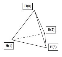
Each point in this solid represents an exchangeable measure on the sequence of three draws. The vertices mark the pure Bernoullian probabilities, in which full weight is given to one or another hypothesis H_i. The indifference measure that assigns equal probability 1/4 to each hypothesis is the center of mass of the tetrahedron. As we draw successively (with replacement) from the urn, updating as above, exchangeable beliefs, given by the conditional probabilities

b[R_{(n + 1)} | A(n, k)]

move within the solid. Drawing a red on the first draw puts beliefs before the second draw in the center of mass of the plane bounded by H₁, H₂, and H₃. If a black is drawn on the second draw then conditional beliefs are on the line connecting H₁ and H₂. Continued draws will move conditional beliefs along this line.Suppose now that we continue to draw with replacement, and that A(n,k), with increasing n, is the sequence of draws. Maintaining exchangeability and updating assures that as the number n of draws increases without bound, conditional beliefs

b[R_{(n + 1)} | A(k, n)]

are practically certain to converge to one of the Bernoullian measures

b(R | H_i)

The Bayesian method thus provides a solution to the problem of induction as de Finetti formulated it.

5.3.3 Exchangeability

We gave a definition of exchangeability: Every sequence of the same length with the same frequency of reds has the same probability. In fact, for given k and n, this probability is always equal to the probability of k reds followed by n−k blacks,

b(R1, …, Rk, Bk+1, …, Bn)

=

b(n, k)

/

(

n k

)

(where b(n, k) = the probability of k reds in n trials, in some order or other) for, in the exchangeable case, probability is invariant for permutations of trials. There are alternative definitions: First, it follows from the first definition that

b(R₁, …, R_n) = b(n, n)

and this condition is also sufficient for exchangeability. Finally, if the concept of exchangeability is extended to random variables we have that a sequence {x_i} of random variables is exchangeable if for each n the mean μ(x₁, …, x_n) is the same for every x₁, …, x_n. (See the supplementary document basic probability.)

The above urn example consists of an objective system—an urn containing balls—that is known. Draws from such an urn are random because the precise prediction of the outcomes is very difficult, if not impossible, due to small perturbing causes (the irregular agitation of the balls) not under our control. But in the three-ball example, because there are just four possible contents, described in the four hypotheses, the perturbations don't affect the fact that there are just eight possible outcomes. As the number of balls increases we add hypotheses, but the basic structure remains; our beliefs continue to be exchangeable and the de Finetti representation theorem assures that the probability of drawing k reds in n trials is always expressed in a formula

b(n, k) = ∑_i h_i {p_i(R)^k[1 − p_i(R)]^{(n − k)}}

where the h_i give the probabilities of the hypotheses H_i. In the simple urn example, this representation has the very nice property that its components match up with features of the objective urn system: Each value of p_i corresponds to a constitution of the urn in which the proportion of red balls is p_i, and each h_i is the probability of that constitution as described in the hypothesis H_i. Epistemically, the p_i are, as we saw above, conditional probabilities:

p_i(X) = b(X | H_i)

that express belief in X given the hypothesis H_i about the constitution.

The critical role of the objective situation in applications of exchangeability becomes clear when we reflect that, as Persi Diaconis puts it, to make use of exchangeability one must believe in it. We must believe in a foundation of stable causes (solidity, number, colors of the balls; gravity) as well as in a network of variable and accidental causes (agitation of the balls, variability in the way they are grasped). There are, in Hume's phrase, “a mixture of causes among the chances, and a conjunction of necessity in some particulars, with a total indifference in others” (Hume 1888, 125f.). It is this entire objective system that supports exchangeability. The fundamental causes must be stable and constant from trial to trial. The variable and accidental causes should operate independently from trial to trial. To underscore this Diaconis gives the example of a basketball player practicing shooting baskets. Since his aim improves with continued practice, the frequency of success will increase and the trials will not be exchangeable; the fundamental causes are not stable. Indeed, de Finetti himself warns that “In general different probabilities will be assigned, depending on the order; whether it is supposed that one toss has an influence on the one which follows it immediately, or whether the exterior circumstances are supposed to vary” (de Finetti 1964, 121).

We count on the support of objective mechanisms even when we cannot formulate even vague hypotheses about the stable causes that constitute it. De Finetti gives the example of a bent coin, deformed in such a way that before experimenting with it we have no idea of its tendency to fall heads. In this case our prior beliefs are plausibly represented by a “flat” distribution that gives equal weight to each hypothesis, to each quantity in the [0, 1] interval. The de Finetti theorem says that in this case the probability of k heads in n tosses is

b(n, k)

=

∫

(

n k

)

pk(1 − p)(n−k)f(p)d(p)

where f(p) gives the weights of the different Bernoullian probabilities (hypotheses) p. We may remain ignorant about the stable causes (the shape and distribution of the mass of the coin, primarily) even after de Finetti's method applied to continued experiments supports conditional beliefs about the strength of the coin's tendency to fall heads. We may insist that each Bernoullian probability, each value for p, corresponds to a physical configuration of the coin, but, in sharp contrast to the urn example, we can say little or nothing about the causes on which exchangeability depends. We believe in exchangeability because we believe that whatever those causes are they remain stable through the trials while the variable causes (such as the force of the throw) do not.

5.3.4 Meta-inductions

Suppose that you are drawing with replacement from an urn containing a thousand balls, each either red or black, and that you modify beliefs according to the de Finetti formula

b[R_{(k + 1)} | A(k, n)] = ∑_i h_i[b(A(k, n) | R_j)b(R_j | H_i)]

where the h_i give the probabilities of the updated 1001 hypotheses about the constitution of the urn. Suppose, however, that unbeknownst to you each time a red ball is drawn and replaced a black ball is withdrawn and replaced with a red ball. (This is a variation of the Polya urn in which each red ball drawn is replaced and a second red ball added.)

Without going into the detailed calculation it is evident that your exchangeable beliefs are in this example not supported. To use exchangeability one must believe in it, and to use it correctly, one might add, that belief must be true; de Finettian induction requires a prior assumption of exchangeability.

Obviously no sequence of reds and blacks could provide evidence for the hypothesis of exchangeability without calling it into question; exchangeability entails that any sequence in which the frequency of reds increases with time has the same probability as any of its permutations. The assumption is however contingent and ampliative and should be subject to inductive support. It is worth recalling Kant's thesis, that regularity of succession in time is the schema, the empirical manifestation, of causal connection. From this point of view, exchangeability is a precise contrary of causality, for its “schema”, its manifestation, is just the absence of regularity of succession, but with constant relative frequency of success. The hypothesis of exchangeability is just that the division of labor between the stable and the variable causes is properly enforced; that the weaker force of variable causes acting in the stable setting of fundamental causes varies order without varying frequency. In the case of gambling devices and similar mechanisms we can provide evidence that the fundamental and determining causes are stable: We can measure and weigh the balls, make sure that none are added or removed between trials, drop the dice in a glass of water, examine the mechanism of the roulette wheel. In less restricted cases—aircraft and automobile accidents, tables of mortality, consumer behavior—the evidence is much more obscure and precarious.

5.4 Testing statistical hypotheses

A statistical hypothesis states the distribution of some random variable. (See the supplementary document basic probability for a brief description of random variables.) The support of statistical hypotheses is thus an important sort of inductive inference, a sort of inverse inference. In a wide class of cases the problem of induction amounts to the problem of formulating good conditions for accepting and rejecting statistical hypotheses. Two specific approaches to this question are briefly surveyed here; the method of likelihood ratios and that of Neyman-Pearson statistics. Likelihood can be given short shrift since it is treated in depth and detail in the article on inductive logic. General methodological questions about sampling and the separation of effects are ignored here. What follows are brief descriptions of the inferential structures.

Logical, frequentist, and subjectivistic views of induction presuppose specific accounts of probability. Accounts of hypothesis testing on the other hand do not typically include specific theories of probability. They presume objective probabilities but they depend only upon the commonly accepted laws of probability and upon classical principles relating probabilities and frequencies.

5.4.1 Likelihood ratios and the law of likelihood

If h is a hypothesis and e an evidence statement then the likelihood of h relative to e is just the probability of e conditional upon h:

L(h | e) = P(e | h)

Likelihoods are in some cases objective. If the hypothesis implies the evidence then it follows from the laws of probability that the likelihood L(h | e) is one. Even when not completely objective, likelihoods tend to be less relative than the corresponding confirmation values: If we draw a red ball from an urn of unknown constitution, we may have no very good idea of the extent to which this evidence confirms the hypothesis that 2/3 of the balls in the urn are red, but we don't doubt that the probability of drawing a red ball given the hypothesis is 2/3. (See inductive logic, section 3.1.)

Isolated likelihoods are not good indicators of inductive support; e may be highly probable given h without confirming h. (If h implies e, for example, then the likelihood of h relative to e is 1, but P(h | e) may be very small.) Likelihood is however valuable as a method of comparing hypotheses: The likelihood ratio of hypotheses g and h relative to the same evidence e is the quotient

L(g | e) / L(h | e)

Likelihood ratios may have any value from zero to infinity inclusive. The law of likelihood says roughly that if L(g | e) > L(h | e) then e supports g better than it does h. (See section 3.2 of the article on inductive logic for a more precise formulation.)

The very general intuition supporting the method of likelihood ratios is just inference to the best explanation; accept that hypothesis among alternatives that best accounts for the evidence. Likelihoods figure importantly in Bayesian inverse inference.

5.4.2 Significance tests

Likelihood ratios are a way of comparing competing statistical hypotheses. A second way to do this consists of precisely defined statistical tests. One simple sort of test is common in testing medications: A large group of people with a disease is treated with a medication. There are then two contradictory hypotheses to be evaluated in the light of the results:

h₀: The medication has no effect. (This is the null hypothesis.)

h₁: The medication has some curative effect. (This is the alternative hypothesis.)

Suppose that the known probability of a spontaneous cure, in an untreated patient, is p_c, that the sample has n members, and that the number of cures in the sample is k_e. Suppose further that sampling has been suitably randomized so that the sample of n members has the structure of n draws without replacement from a large population. If the diseased population is very large in comparison with the size n of the sample, then draws without replacement are approximated by draws with replacement and the sample can be treated as a collection of independent and equiprobable trials. In this case, if C is a group of n untreated patients, for each k between zero and n inclusive the probability of k cures in C is given by the binomial formula:

P(k cures in C)	=	b(n, k, pc)
	=	(	n k	)	pck(1−pc)(n−k)

If the null hypothesis, h₀, is true we should expect the probability of k cures in the sample to be the same:

P(k cures in the sample | h0)	=	P(k cures in C)
	=	b(n, k, pc)
	=	(	n k	)	pck(1−pc)(n−k)

Let k_c = p_cn. This is the expected number of spontaneous cures in n untreated patients. If h₀ is true and the medication has no effect, k_e (the number of cures in the medicated sample) should be close to k_c and the difference

k_e − k_c

(known as the observed distance) should be small. As k varies from zero to n the random variable

k − k_c

takes on values from −k_c to n−k_c with probabilities

b(n, 0, p_c), b(n, 1, p_c), …, b(n, n, p_c)

This binomial distribution has its mean at k = k_c, and this is also the point at which b(n, k, p_c) reaches its maximum. A histogram would look something like this.

Distribution of k − k_c

Given p_c and n, this distribution gives the probability that the observed distance has the different possible sizes between its minimum, −k_c, and its maximum at n−k_c; probabilities of the different values of k−k_c are on the abscissa. The significance level of the test is the probability given h₀ of a distance as large as the observed distance.

A high significance level means that the observed distance is relatively small and that it is highly likely that the difference is due to chance, i.e. that the probability of a cure given medication is the same as the probability of a spontaneous, unmedicated, cure. In specifying the test an upper limit for the significance level is set. If the significance level exceeds this limit, then the result of the test is confirmation of the null hypothesis. Thus if a low limit is set (limits on significance levels are typically .01 or .05, depending upon cost of a mistake) it is easier to confirm the null hypothesis and not to accept the alternative hypothesis. Caeteris paribus, the lower the limit the more severe the test; the more likely it is that P(cure | medication) is close to p_e = k_e / n.

This is not the place for an extended methodological discussion, but one simple principle, obvious upon brief reflection, should be mentioned. This is that the size n of the sample must be fixed in advance. Else a persistent researcher could, with arbitrarily high probability, obtain any ratio p_e = k_e / n and hence any observed difference k_e − k_c desired; for, in the case of Bernoulli trials, for any frequency p the probability that at some n the frequency of cures will be p is arbitrarily close to one.

5.4.3 Power, size, and the Neyman-Pearson lemma

If h is any statistical hypothesis a test of h can go wrong in either of two ways: h may be rejected though true—this is known as a type I error; or it may be accepted though false—this is a type II error.

If f is a (one-dimensional) random variable that takes on values in some interval of the real line with definite probabilities and h is a statistical hypothesis that determines a probability distribution over the values of f, then a pure statistical test of h specifies an experiment that will yield a value for f and specifies also a region of values of f—the rejection region of the test. If the result of the experiment is in the rejection region, then the hypothesis is rejected. If the result is not in the rejection region, the hypothesis is not rejected. A mixed statistical test of a hypothesis h includes a pure test but in addition divides the results not in the rejection region into two sub-regions. If the result is in the first of these regions the hypothesis is not rejected. If the result is in the second sub-region a further random experiment, completely independent of the first experiment, but with known prior probability of success, is performed. This might be, for example, drawing a ball from an urn of known constitution. If the outcome of the random experiment is success, then the hypothesis is not rejected, otherwise it is rejected. Hypotheses that are not rejected may not be accepted, but may be tested further. This way of looking at testing is quite in the spirit of Popper. Recall his remark that

The best we can say of a hypothesis is that up to now it has been able to show its worth, and that it has been more successful than other hypotheses although, in principle, it can never be justified, verified, or even shown to be probable. This appraisal of the hypothesis relies solely upon deductive consequences (predictions) which may be drawn from the hypothesis … (Popper 1959, 315)

A hypothesis that undergoes successive and varied statistical tests shows its worth in this way. Popper would not call this process “induction”, but statistical tests are now commonly taken to be a sort of induction.

Given a statistical test of a hypothesis h two critical probabilities determine the merit of the test. The size of the test is the probability of a type I error; the probability that the hypothesis will be rejected though true; and the power of the test is the chance of rejecting h if it is false. A good test will have small size and large power.

size = Prob(reject h and h is true)

power = Prob(reject h and h is false)

The fundamental lemma of Neyman-Pearson asserts that for any statistical hypothesis of any given size, there is a unique test of maximum power (known as a best test of that size). The best test may be a mixed test, and this is sometimes said to be counterintuitive: A mixed test (tossing a coin, drawing a ball from an urn) may, as Mayo puts it, “even be irrelevant to the hypothesis of interest” (Mayo 1996, 390). Mixed tests bear an uncomfortable resemblance to consulting tea leaves. Indeed, recent exponents of the Neyman-Pearson approach favor versions the theory that do not depend on mixed tests (Mayo 1996, 390 n.).

6. Induction, Values, and Evaluation

6.1 Pragmatism: induction as practical reason

In 1953 Richard Rudner published “The Scientist qua Scientist Makes Value Judgments” in which he argued for the thesis expressed in its title. Rudner's argument was simple and can be sketched in the framework of the Neyman-Pearson model of hypothesis testing: “[S]ince no hypothesis is ever completely verified, in accepting a hypothesis the scientist must make the decision that the evidence is sufficiently strong or that the probability is sufficiently high to warrant the acceptance of the hypothesis.” (Rudner 1953, 2) Sufficiency in such a decision will and should depend upon the importance of getting it right or wrong. Tests of hypotheses about the quality of a “lot of machine stamped belt buckles” may and should have smaller size and larger power than those about drug toxicity. The argument is not restricted to scientific inductions; it shows as well that our everyday inferences depend inevitably upon value judgments; how much evidence one collects depends upon the importance of the consequences of the decision.

Isaac Levi in responding to Rudner's claim, and to later formulations of it, distinguished cognitive values from other sorts of values; moral, aesthetic, and so on. (Levi 1986, 43–46) Of course the scientist qua scientist, that is to say in his scientific activity, makes judgments and commitments of cognitive value, but he need not, and in many instances should not, allow other sorts of values (fame, riches) to weigh upon his scientific inductions.

What is in question is the separation of practical reason from theoretical reason. Rudner denies the distinction; Levi does too, but distinguishes practical reason with cognitive ends from other sorts. Recent pragmatic accounts of inductive reasoning are even more radical. Following (Ramsey 1926) and (Savage 1954) they subsume inductive reasoning under practical reason; reason that aims at and ends in action. These and their successors, such as (Jeffrey 1983), define partial belief on the basis of preferences; preferences among possible worlds for Ramsey, among acts for Savage, and among propositions for Jeffrey. (See section 3.5 of interpretations of probability). Preferences are in each case highly structured. In all cases beliefs as such are theoretical entities, implicitly defined by more elaborate versions of the pragmatic principle that agents (or reasonable agents) act (or should act) in ways they believe will satisfy their desires: If we observe the actions and know the desires (preferences) we can then interpolate the beliefs. In any given case the actions and desires will fit distinct, even radically distinct, beliefs, but knowing more desires and observing more actions should, by clever design, let us narrow the candidates.

In all these theories the problem of induction is a problem of decision, in which the question is which action to take, or which wager to accept. The pragmatic principle is given a precise formulation in the injunction to act so as to maximize expected utility, to perform that action, A_i among the possible alternatives, that maximizes

U(A_i) = ∑j P(S_j | A_i)U(S_j A_i)

where the S_j are the possible consequences of the acts A_i, and U gives the utility of its argument.

6.2 On the value of evidence

One significant advantage of this development is that the cost of gathering more information, of adding to the evidence for an inductive inference, can be factored into the decision. Put very roughly, the leading idea is to look at gathering evidence as an action on its own. Suppose that you are facing a decision among acts A_i, and that you are concerned only about the occurrence or non-occurrence of a consequence S. The principle of utility maximization directs you to choose that act A_i that maximizes

U(A_i) = ∑j P(S_j | A_i)U(S_j A_i)

where the S_j are the possible consequences of the acts A_i

Suppose further that you have the possibility of investigating to see if evidence E, for or against S, obtains. Assume further that this investigation is cost-free. Then should you investigate and find E to be true, utility maximization would direct you to choose that act A_i that maximizes utility when your beliefs are conditioned on E:

U_E(A_i) = P(S | E A_i)U(S E A_i) + P(¬S | E A_i)U(¬S E A_i)

And if you investigate and find E to be false, the same principle directs you to choose A_i to maximize utility when your beliefs are conditioned on ¬E:

U_¬E(A_i) = P(S | ¬E A_i)U(S ¬E A_i) + P(¬S | ¬E A_i)U(¬S ¬E A_i)

Hence if your prior strength of belief in the evidence E is P(E), you should choose A_i to maximize the weighted average

P(E)U_E(A_i) + P(¬E)U_¬E(A_i)

and if the maximum of this weighted average exceeds the maximum of U(A_i), then you should investigate. About this several brief remarks:

• Notice that the utility of investigation depends upon your beliefs about your future beliefs and desires, namely that you believe now that following the investigation you will maximize utility and update your beliefs.
• Investigation is in the actual world normally not cost-free. It takes time, trouble, sometimes money, and is sometimes dangerous. A general theory of epistemic utility should consider these factors.
• I. J. Good (Good 1967) proved that in the cost-free case U(A_i) can never exceed U_E(A_i) and that when the utilities of outcomes are distinct the latter always exceeds the former (Skyrms 1990, chapter 4).
• The question of bad evidence is critical. The evidence gathered might take you further from the truth. (Think of drawing a succession of red balls from an urn containing predominantly blacks.)

7. Justification and Support of Induction

7.1 Hume's dilemma revisited

The question of justification for induction, mentioned in the introduction, was postponed to follow discussion of several approaches to the problem. We can now revisit this matter in the light of the intervening accounts of induction.

Hume's simple argument for the impossibility of a justification of induction is a dilemma: Any justification must be either deductive or inductive. Whatever is established deductively is necessarily true, but inductions are never necessarily true, so no deductive justification of induction is possible. Inductive justification of induction, on the other hand would be circular, since it would presume the very justification that it pretends to provide. Induction is hence unjustifiable.

We remarked that Hume himself qualifies this conclusion. Wise men, he says, review their inferences and reflect upon their reliability. This review may lead us to correct our present inductive reasoning in view of past errors: noting that I've persistently misestimated the chances of rain, I may revise my forecast for tomorrow. The process is properly speaking not circular but regressive or hierarchical; a meteorological induction is reviewed by an induction not about meteorology but about inductions. Notice also that revision of the forecast of rain will not typically consist in reducing the chance of rain (and concomitantly increasing strength of belief in fair weather). The most plausible and common revision is rather, to put it in modern terms, an increase in dispersion: What was a pointed forecast of 2/3 becomes a vague interval of belief, from about (say) 1/2 to 3/4. This uncertainty will propagate up the hierarchy of inductions: Reflection leads me to be less certain about my reasoning about weather forecasts. Continuing the process must, in Hume's elegant phrase, “weaken still further our first evidence, and must itself be weaken'd by a fourth doubt of the same kind, and so on in infinitum”. How is it then that our cognitive faculties are not totally paralyzed? How do we “retain a degree of belief, which is sufficient for our purpose, either in philosophy or in common life?”(Hume 1888, 182, 185) How do we ever arrive at beliefs about the weather, not to speak of the laws of classical physics?

7.1.1 General rules and higher-order inductions

Hume's resolution of this puzzle is in terms of general rules, rules for judging (Hume 1888, 150). These are of two sorts. Rules of the first sort triggered by the experience of successive instances lead to singular predictive inferences . These when unchecked may tempt us to wider and more varied predictions than the evidence supports (to grue-type inferences, for example). Rules of the second sort are corrective, these lead us to correct and limit the application of rules of the first sort on the basis of evidence of their unreliability. It is only by following general rules, says Hume, that we can correct their errors.

Recall that Reichenbach gave an account of higher order or, as he called them, concatenated, probabilities in terms of arrays or matrices. The second-order probability

P {[P(C | B) = p] | A} = q

is defined as the limit of a sequence of first order probabilities. This gives a way in a Reichenbachean framework of inductively evaluating inductions in a given class or sort. Reichenbach refers to this as the self-corrective method, and he cites Peirce, “who mentioned ‘the constant tendency of induction to correct itself’”, as a predecessor (Reichenbach 1971, 446 n., Peirce 1935, vol II 456). Peirce consistently thinks this way: “Given a certain state of things, required to know what proportion of all synthetic inferences relating to it will be true within a given degree of approximation” (Peirce 1955, 184). Ramsey cites Mill approvingly for “his way of treating the subject as a body of inductions about inductions” (Ramsey 1931, 198). See, e.g. (Mill 2002, 209) “This is a kind of pragmatism:” Ramsey writes, “we judge mental habits by whether they work, i.e., whether the opinions they lead to are for the most part true” (Ramsey 1931, 197–198). Hume went so far as to give a set of eight “Rules by which to judge of causes and effects” (Hume 1888, I.III.15), obvious predecessors of Mill's canons.

7.2 Induction and deduction

If the inductive support of induction need not be simply circular, the deductive support of induction is also seen, upon closer examination, not to be as easily dismissed as the dilemma might make it seem. The laws of large numbers, the foundation of inductive inferences relating frequencies and probabilities, are mathematical consequences of the laws of probability and hence necessary truths. Of course the application of these laws in any given empirical situation will require contingent assumptions, but the essentially inductive part of the reasoning certainly depends upon the deductively established laws.

The dilemma—inductive support for induction would be circular, deductive support is impossible—thus turns out to be less simple than it at first appears. The application of induction to inductive inference is neither circular nor justificatory. It is hierarchical and corrective. Statistical inferences based on the laws of large numbers depend essentially upon the deductive support for those laws.

7.3 Assessing the reliability of inductive inferences: calibration

These considerations suggest deemphasizing the question of justification—show that inductive arguments lead from truths to truths—in favor of exploring methods to assess the reliability of specific inferences. How is this to be done? If after observing repeated trials of a phenomenon we predict success of the next trial with a probability of 2/3, how is this prediction to be counted as right or wrong? The trial will either be a success or not; it can't be two-thirds successful. The approach favored by the thinkers mentioned above is to evaluate not individual inferences or beliefs, but habits of forming such beliefs or making such inferences.

One method for checking on probabilistic inferences can be illustrated in probabilistic weather predictions. Consider a weather forecaster who issues daily probabilistic forecasts. For simplicity of illustration suppose that only predictions of rain are in question, and that there are just a few distinct probabilities (e.g., 0, 1/10, …, 9/10, 1). We say that the forecaster is perfectly calibrated if for each probability p, the relative frequency of rainy days following a forecast of rain with probability p is just p, and that calibration is better as these relative frequencies approach the corresponding probabilities. Without going into the details of the calculation, the rationale for calibration is clear: For each probability p we treat the days following a forecast of probability p as so many Bernoulli trials with probability p of success. The difference between the binomial quotient and p then measures the goodness of calibration; the smaller the difference the better the calibration.

This account of calibration has an obvious flaw: A forecaster who knows that the relative frequency of rainy days overall is p can issue a forecast of rain with probability p every day. He will then be perfectly calibrated with very little effort, though his forecasts are not very informative. The standard way to improve this method of calibration was designed by Glenn Brier in (Brier 1950). In addition to calibrating probabilities with relative frequencies it weights favorably forecast probabilities that are closer to zero and one. The method can be illustrated in the case of forecasts with two possible outcomes, rain or not. If there are n forecasts, let p_i be the forecast probability of rain on trial i, q_i = (1 − p_i), 1 ≤ i ≤ n, and let E_i be a random variable which is one if outcome i is rain and zero otherwise. Then the Brier Score for the n forecasts is

B = (1/n)∑_i(p_i − E_i)²(q_i − E_i)²

Low Brier scores indicate good forecasting: The minimum is reached when the forecasts are all either zero or one and all correct, then B = 0. The maximum is when the forecasts are all either zero or 1 and all in error, then B = 1. More recently the method has been ramified and applied to subjective probabilities in general. See (van Fraassen 1983).

7.4 Why trust induction? The question revisited

We can now return to the general question posed in section 1: Why trust induction more than other methods? Why not consult sacred writings, or “the wisdom of crowds” to explain and predict the movements of the planets, the weather, automotive breakdowns or the evolution of species?

7.4.1 The wisdom of crowds

The wisdom of crowds can appear to be an alternative to induction. James Surowiecki argued, in the book of this title (Surowiecki, 2004) with many interesting examples that groups often make better decisions than even informed individuals. It is important to emphasize that the model requires independence of the individual decisions and also a sort of diversity to assure that different sources of information are at work, so it is to be sharply distinguished from judging the mass opinion of a group that reaches a consensus in discussion. The obvious method suggested by Surowiecki's thesis is to consult polls or predictions markets rather than to experiment or sample on one's own. (See, for example, http://www.chrisfmasse.com/ for an account of predictions markets.)

There is in fact a famous classical theorem, not mentioned by Surowiecki, that gives a precise rationale for the wisdom of crowds. This is the Condorcet Jury theorem, first proved by Condorcet (1743–1794). (See Black 1963, 164f. for a perspicuous proof.) The import of the theorem can be expressed as follows:

Suppose that a group of people each expresses a yes-no opinion about the same matter of fact, that they reach and express these opinions independently, and that each has better than 50% chance of being right. Then as the size of the group increases without bound the probability that a majority will be right approaches one.

(The condition can be weakened; probabilities need not uniformly exceed 50%. Again, it also applies to quantitative estimates in which more than two possible values are in question.) To see why the theorem holds, consider a very simple special case in which everyone has exactly 2/3 probability of being right. Amalgamating the opinions then corresponds to drawing with replacement once from each urn in a collection in which each urn contains two red (true) balls and one black (false) ball. The (weak) law of large numbers entails that as the number of urns, and hence draws, increases without bound the probability that the relative frequency of reds (or true opinions) differs from 2/3 by a fixed small quantity approaches zero. (See the supplementary document Basic Probability.) This also underscores the importance of the diversity requirement; if everyone reached the same conclusion on the basis of the same sources, however independently, the conclusion would be no better supported than that reached by any individual. And, of course, the requirement that the probabilities (or a sufficient number of them) exceed 50% is critical: If these probabilities are all less than 50% the theorem implies that a majority will be wrong. The method of the wisdom of crowds depends in this way upon reliable reasoning by the members of the crowd. Good or bad individual reasoning translates into good or bad reasoning on the part of the crowd. Clearly, the wisdom of crowds is not to be contrasted with inductive reasoning, indeed it depends upon the inductive principle expressed in the Condorcet theorem to amalgamate correctly the individual testimonies as well as upon the diversity of individual reasonings. What is valuable in the method is the diversity of ways of forming beliefs. This amounts to a form of the requirement of total evidence, briefly discussed in section 3.3 above.

As with Reichenbach's account of single-case probabilities, the wisdom of crowds depends essentially upon testimony.

7.4.2 Creationism and Intelligent Design

The wisdom of crowds thus depends upon good inductive reasoning. The use of sacred writings or other authorities to support judgments about worldly matters is, however, another matter. Christian Creationism, a collection of views according to which the biblical myth of creation, primarily as found in the early chapters of the book of Genesis, explains, either in literal detail or in metaphorical language, the origins of life and the universe, is perhaps the most popular alternative to accepted physical theory and the Darwinian account of life forms in terms of natural selection. (See (Ruse 2005) and the entry on creationism). Christian Creationism, nurtured and propagated for the most part in the United States, contradicts inductively supported scientific theories, and depends not at all upon any recognizable inductive argument. Many of us find it difficult to take the view seriously, but, according to recent investigations: "Over the past 20 years, the percentage of U.S. adults accepting the idea of evolution has declined from 45% to 40% and the percentage of adults overtly rejecting evolution declined from 48% to 39%. The percentage of adults who were not sure about evolution increased from 7% in 1985 to 21% in 2005" (Miller et al. 2006, 766).

The apparent absurdity of Creationism has led some opponents of evolutionism and the doctrine of natural selection to eschew biblical forms of the view and to formulate a weaker thesis, known as Intelligent Design (Behe 1996, Dembski 1998). Intelligent design cites largely unquestioned evidence of two sorts: The delicate balance—that even a minute change in any of many physical constants would tip the physical universe into disequilibrium and chaotic collapse; and the complexity of life—that life forms on earth are very complex. The primary thesis of Intelligent Design is that the hypothesis of a designing intelligence explains these phenomena better than do current physical theories and Darwinian natural selection.

Intelligent Design is thus not opposed to induction. Indeed its central argument is frankly inductive, a claim about likelihoods:

P(balance and complexity | Intelligent Design) >
P(balance and complexity | current physics and biology)

There are a number of difficulties with Intelligent Design, explained in detail by Elliott Sober in (Sober 2002). (This article also includes an excellent primer on the sorts of probabilistic inference involved in the likelihood claim. See also the article on Creationism. Briefly put, there are problems of two sorts, both clearly put in Sober's article: First, Intelligent Design theorists “don't take even the first steps towards formulating an alternative theory of their own that confers probabilities on what we observe” as the likelihood principle would require (75). Second, the Intelligent Design argument depends upon a probabilistic fallacy. The biological argument, to restrict consideration to that, infers from

Prob(organisms are very complex | evolutionary theory) = low
Organisms are very complex

To

Prob(evolutionary theory) = low

To see the fallacy, compare this with

Prob(double zero | the roulette wheel is fair) = low
Double zero occurred

Thus, Prob(the wheel is fair) = low

What is to be emphasized here, however, is not the fallaciousness of the arguments adduced in favor of Intelligent Design. It is that Intelligent Design, far from presenting an alternative to induction, presumes certain important inductive principles.

7.4.3 Induction and testimony

Belief based on testimony, from the viewpoint of the present article, is not a form of induction. A testimonial inference has typically the form:

An agent A asserts that X

A is reliable

Therefore, X

Or, in a more general probabilistic form:

An agent A asserts that X

For any proposition X Pr(X | A asserts that X) = p

Pr(X) = p

In an alternative form the asserted content is quoted directly.

What is characteristic and critical in inference based on testimony is the inference from a premise in which the conclusion is expressed indirectly, in the context of the agent's assertion (A asserts that X), to a conclusion in which that content occurs directly, not mediated by language or mind (X). It is also important that testimony is always the testimony of some agent or agents. And testimonial inference is not causal; testimony is neither cause not effect of what is testified to. This is not to say that testimonial inference is less reliable than induction; only that it is different.

Although testimonial inference may not be inductive, induction would be all but paralyzed were it not nourished by the testimony of authorities, witnesses, and sources. We hold that causal links between tobacco and cancer are well established by good inductive inferences, but the manifold data come to us through the testimony of epidemiological reports and, of course, texts that report the establishment of biological laws. Kepler's use of Tycho's planetary observations is a famous instance of induction based on testimony. Reichenbach's frequentist account of single-case probabilities as well as the wisdom of crowds require testimonial inference as input for their amalgamating inductions. And actuaries, those virtuosi of inductivism, depend entirely upon reports of data to base their conclusions. Of course inductive inferences from testified or reported data are no more reliable than the data.

7.5 Learning to love induction

There are really two questions here: Why trust specific inductive inferences? and Why trust induction as a general method? The response to the first question is: Trust specific inductions only to the extent that they are inductively supported or calibrated by higher-order inductions. It is a great virtue of Ramsey's counsel to treat “the subject as a body of inductions about inductions” that it opens the way to this. As concerns trust in induction as a general method of forming and connecting beliefs, induction is not all that easy to avoid; the wisdom of crowds and Intelligent Design seem superficially to be alternatives to induction, but both turn out upon closer examination to be inductive. Induction is, after all, founded on the expectation that characteristics of our experience will persist in experience to come, and that is a basic trait of human nature. “Nature”, writes Hume, “by an absolute and uncontroulable necessity has determin'd us to judge as well as to breathe and feel” (Hume 1888, 183). “We are all convinced by inductive arguments”, says Ramsey, “and our conviction is reasonable because the world is so constituted that inductive arguments lead on the whole to true opinions. We are not, therefore, able to help trusting induction, nor, if we could help it do we see any reason why we should” (Ramsey 1931, 197). We can, however, trust selectively and reflectively; we can winnow out the ephemera of experience to find what is fundamental and enduring.

The great advantage of induction is not that it can be justified or validated, as can deduction, but that it can, with care and some luck, correct itself, as other methods do not.

7.6 Naturalized and evolutionary epistemology

“Our reason”, writes Hume, “must be consider'd as a kind of cause, of which truth is the natural effect; but such-a-one as by the irruption of other causes, and by the inconstancy of our mental powers, may frequently be prevented” (Hume 1888, 180).

Perhaps the most robust contemporary approaches to the question of inductive soundness are naturalized epistemology and its variety evolutionary epistemology. These look at inductive reasoning as a natural process, the product, from the point of view of the latter, of evolutionary forces. An important division within naturalized epistemology exists between those who hold that there is little or no role in the study of induction for normative principles; that a distinction between correct and incorrect inductive methods has no more relevance than an analogous distinction between correct and incorrect species of mushroom; and those for whom epistemology should not only describe and categorize inductive methods but also must evaluate them with respect to their success or correctness.

The encyclopedia entries on these topics provide a comprehensive introduction to them.

Bibliography

• Achinstein, Peter. 1963. “Variety and Analogy in Confirmation Theory.” Philosophy of Science, 30: 207 - 221.
• Adams, Ernest. 1965. “A Logic of Conditionals.” Inquiry, 8: 166-97.
• –––. 1975. The Logic of Conditionals. Dordrecht: Reidel.
• –––. 1966. “Probability and the Logic of Conditionals.” In Aspects of Inductive Logic, edited by Jaakko Hintikka, Amsterdam: North Holland, 256–316.
• –––. 1970. “Subjunctive and Indicative Conditionals.” Foundations of Language 6/1: 89-94.
• Black, Duncan. 1963. The Theory of Committees and Elections. Cambridge: Cambridge University Press.
• Brier, Glenn. 1950, “Verification of Forecasts Expressed in Terms of Probability.” Monthly Weather Review 78/1: 1–3.
• Carnap, Rudolf. 1952. The Continuum of Inductive Methods. Chicago: The University of Chicago Press.
• –––. 1962. Logical Foundations of Probability. second ed. Chicago: University of Chicago Press.
• Carnap, Rudolf, and Jeffrey, Richard, eds. 1971 (1980). Studies in Inductive Logic and Probability. Berkeley and Los Angeles: University of California Press, 2 volumes.
• Cramer, Harald. 1955. The Elements of Probability Theory. New York, London: John Wiley and Sons.
• de Finetti, Bruno. 1964. “Foresight: Its Logical Laws, Its Subjective Sources.” In Studies in Subjective Probability, edited by Henry E. Kyburg and Howard E. Smokler. New York, London, Sydney: John Wiley and Sons.
• –––. 1974 (1975). The Theory of Probability: A Critical Introductory Treatment. Translated by Antonio Machi and Adrian Smith. (Wiley Series in Probability and Mathematical Statistics), London, New York: John Wiley and Sons, 2 volumes.
• di Maio, Maria Concerta. 1995. “Predictive Probability and Analogy by Similarity in Inductive Logic.” Erkenntnis, 43: 369–94.
• Feller, William. 1950 (1966). An Introduction to Probability Theory and Its Applications. New York, London: John Wiley and Sons, 2 volumes.
• Glymour, Clark. 2001. “Instrumental Probability.” The Monist 84/2: 284–300.
• Good, I. J. 1967. “On the Principle of Total Evidence.” British Journal for the Philosophy of Science, 17: 319–21.
• Goodman, Nelson. 1965. Fact, Fiction, and Forecast. Indiannapolis, New York: Bobbs Merrill, second edition.
• Grattan-Guinness, I. 2004. “Karl Popper and ‘the Problem of Induction’: A Fresh Look at the Logic of Testing Scientific Theories.” Erkenntnis, 60/1: 107–20.
• Hacking, Ian. 1965. Logic of Statistical Inference. Cambridge: Cambridge University Press.
• Hempel, Carl G. 1945. “Studies in the Logic of Confirmation I.” Mind NS, 54/213: 1–26.
• –––. 1945. “Studies in the Logic of Confirmation Ii.” Mind NS, 54/214: 97–121.
• Hume, David. 1888. Hume's Treatise of Human Nature. Edited by L.A. Selby Bigge. Oxford: Clarendon Press. Originally published 1739–40.
• –––. 1975. Enquiries Concerning Human Understanding and Concerning the Principles of Morals. Oxford: Clarendon Press. Originally published 1748 and 1751.
• Jeffrey, Richard C. 1983. The Logic of Decision. second ed. Chicago and London: University of Chicago Press.
• Juhl, Cory F. 1994. “The Speed-Optimality of Reichenbach's Straight Rule of Induction.” British Journal of the Philosophy of Science, 45/3: 857-63.
• Katz, Jerrold. 1962. The Problem of Induction and Its Solution. Chicago: University of Chicago Press.
• Kolmogorov, Andrei Nikolaevich. 1950. Foundations of the Theory of Probability. Translated by Nathan Morrison (editor). New York: Chelsea Publishing Co.
• Lange, Mark. 1999. “Calibration and the Epistemological Role of Bayesian Conditionalization.” Journal of Philosophy, 96/6: 294–324.
• Levi, Isaac. 1986. Hard Choices. Cambridge: Cambridge University Press.
• Lewis, David. 1983 (1986). Philosophical Papers. New York, Oxford: Oxford University Press, 2 volumes.
• Mayo, Deborah. 1996. Error and the Growth of Experimental Knowledge. Chicago: University of Chicago Press.
• Mellor, D.H., ed. 1980. Prospects for Pragmatism: Essays in Memory of F.P. Ramsey. Cambridge: Cambridge University Press.
• Mill, John Stuart. 2002. A System of Logic: Ratiocinative and Inductive. Honolulu: University Press of the Pacific. Originally published 1843.
• Miller, Jon D., Eugenie C. Scott, Shinji Okamato. 2006. “Public Acceptance of Evolution.” Science, 313/5788, 765–766.
• Parrini, Paolo, Wesley Salmon, and Merrilee Salmon (eds.), 2003. Logical Empiricism, Historical & Contemporary Perspectives. Pittsburgh: University of Pittsburgh Press.
• Peano, Giuseppe. 1973. Selected Works of Giuseppe Peano. Translated by Hubert C. Kennedy. Toronto: University of Toronto Press.
• Pearl, Judea. 2000. Causality: Models, Reasoning, and Inference. Cambridge: Cambridge University Press.
• Peirce, Charles S. 1935 (1961). Collected Papers. Edited by Charles Hartshorne and Paul Weiss. Cambridge, MA: Harvard University Press, 4 volumes.
• –––. 1955. Philosophical Writings of Peirce. Edited by Justus Buchler. New York: Dover Publications.
• Popper, Karl. 1959. The Logic of Discovery. Translated by Author. New York: Basic Books.
• Ramsey, Frank P. 1931. The Foundations of Mathematics and Other Logical Essays, (International Library of Psychology Philosophy and Scientific Method) London: Routledge and Kegan Paul.
• Reichenbach, Hans. 1956. The Direction of Time. Berkeley and Los Angeles: University of California Press.
• –––. 1961. Experience and Prediction. Chicago: The University of Chicago Press.
• –––. 1971. The Theory of Probability. second ed. Berkeley, Los Angeles, London: University of California Press.
• Rudner, Richard. 1953. “The Scientist Qua Scientist Makes Value Judgments.” Philosophy of Science, 20: 1–6.
• Ruse, Michael. 2005. “Methodological Naturalism Under Attack.” South African Journal of Philosophy 24/1: 44–60.
• Salmon, Wesley. 1963. “On Vindicating Induction.” Philosophy of Science, 30/3: 252–61.
• –––. 1967. Foundations of Scientific Inference. Pittsburgh: University of Pittsburgh Press.
• Savage, Leonard J. 1954. The Foundations of Statistics. New York: John Wiley and Sons.
• Scheffler, Israel. 1963. The Anatomy of Inquiry. New York: Alfred A. Knopf.
• Skyrms, Brian. 1986. Choice and Chance: An Introduction to Inductive Logic. Belmont, California: Wadsworth Publishing Company, third edition.
• Skyrms, Brian. 1990. The Dynamics of Rational Deliberation. Cambridge, Massachusetts: Harvard University Press.
• –––. 1994. “Bayesian Projectability.” In Grue: Essays on the New Riddle of Induction, edited by Douglas Stalker. Chicago: Open Court.
• Sober, Elliott. 2002. “Intelligent Design and Probability Reasoning.” International Journal for Philosophy of Religion 52: 65–80.
• Stalker, Douglas. 1994. Grue: Essays on the New Riddle of Induction. Chicago: Open Court.
• Surowiecki, James. 2004. The Wisdom of Crowds: Why the Many Are Smarter Than the Few and How Collective Wisdom Shapes Business, Economies, Societies and Nations. London: Little Brown.
• Vickers, John M. 1988. Chance and Structure: An Essay on the Logical Foundations of Probability. Oxford, Clarendon Press.
• van Fraassen, Bas. 1976. “Representation of Conditional Probabilities.” Journal of Philosophical Logic, 5: 417–30.
• –––. 1983. “Calibration: A Frequency Justification for Personal Probability.” In Physics, Philosophy, and Psychoanalysis, edited by R.S. Cohen and Laudan, Boston: Reidel, 295–319.
• Whitehead, Alfred North. 1948. Science and the Modern World. New York: Macmillan.
• –––. and Bertrand Russell. 1927. Principia Mathematica. Cambridge: Cambridge University Press, 1957, second edition, 3 volumes.

Other Internet Resources

• Teaching Theory of Knowledge: Probability and Induction, organization of topics and bibliography by Brad Armendt (Arizona State University) and Martin Curd (Purdue).

Related Entries

actualism | Bayes' Theorem | Carnap, Rudolf | conditionals | confirmation | epistemology: evolutionary | epistemology: naturalized | fictionalism: modal | Frege, Gottlob: logic, theorem, and foundations for arithmetic | Goodman, Nelson | Hempel, Carl | Hume, David | induction: new problem of | logic: inductive | logic: non-monotonic | memory | Mill, John Stuart | perception: epistemological problems of | Popper, Karl | probability, interpretations of | Ramsey, Frank | Reichenbach, Hans | testimony: epistemological problems of | Vienna Circle

Copyright © 2006 by
John Vickers <John.Vickers@cgu.edu>