|
Stochastic integration 2018-2019 (code 5374STIN8Y) ContentsStochastic calculus is an indispensable tool in modern financial mathematics. In this course we present this mathematical theory. We treat the following topics from martingale theory and stochastic calculus: martingales in discrete and continuous time, the Doob-Meyer decomposition, construction and properties of the stochastic integral, Itô's formula, (Brownian) martingale representation theorem, Girsanov's theorem, stochastic differential equations and we will briefly explain their relevance for mathematical finance.AimsAt the end of the course, students
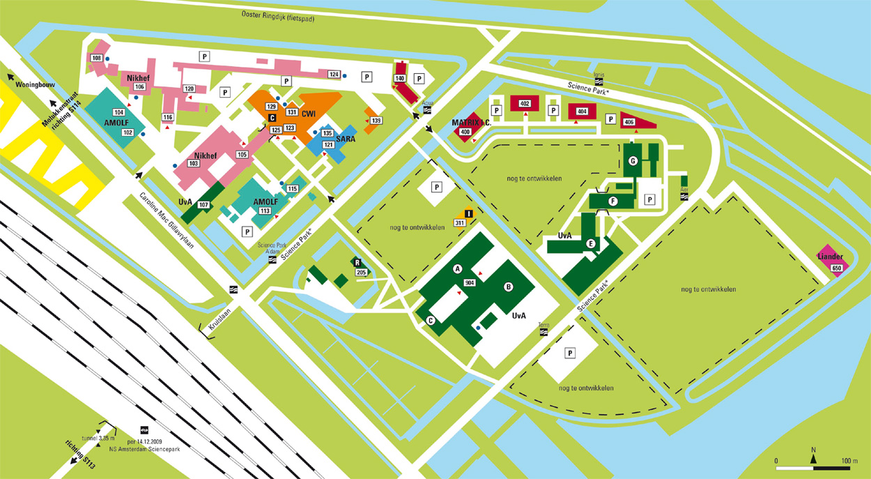
PrerequisitesMeasure theory, stochastic processes at the level of the course Measure Theoretic Probability (2010 version)LiteratureRecommended background reading: I. Karatzas and S.E. Shreve, Brownian motions and stochastic calculus and D. Revuz and M. Yor, Continuous martingales and Brownian motion. The contents of the course are described in the (based on these books) lecture notes.Companion courseIn the past students were recommended to take also the course on Stochastic Processes by Floske Spieksma (UL), see also the Spring Courses of the Dutch Master Program in Mathematics (2018). This course has been replaced with a new one under the same name, but with different topics.Follow up coursesA course that heavily relies on stochastic calculus is Interest rate models (the webpage is a bit outdated, but still fine for a first impression).LecturersAsma Khedher (first half) and Peter Spreij (second half), assistance by Sven Karbach.HomeworkStrict deadlines: the lecture after you have been given the assignment, although serious excuses will always be accepted. You are allowed to work in pairs (a pair means 2 persons, not 3 or more), in which case one set of solutions should be handed in.ScheduleSpring semester: Thursdays, 09:00-10:45, first lecture on Thursday 7 February 2019. Tutorials biweekly after the lectures. For up to date information on the lecture rooms, see datanose.nl. See also the map of Science Park and the travel directions. Changes in the schedule: no lecture and exercises on April 18, 2019.ExaminationThe final grade is a combination of the results of the take home assignments and the written or oral exam (first part, to be decided) and oral exam (second part). Note, added on 29 May 2019: the homework results count as a bonus for 30% of the final grade. The partial oral exams have equal weight.To take the oral exam for the second part, you make an appointment with Peter for a date that suits your own agenda. If it happens that you'd like to postpone the appointment, just inform us that you want so. This is never a problem! The only important matter is that you take the exam, when you feel ready for it. What do you have to know? The theory, i.e. all important definitions and results (lemma's, theorems, etc.). Optional: you may prepare three theorems together with their proofs. You select your favourite ones! Criteria to consider: they should be interesting, non-trivial and explainable in a reasonably short time span. You will be asked to present one of them. Make an appointment with Peter for a date that suits you well. Impossible dates are May 22-31 (perhaps with an exception on May 29), June 3, 6, 10-24, 26, July 23 - August 20. RegistrationThe UvA now wants all participants to be registered four weeks before the start of the course. If you missed this deadline you can use the late registration form. Note that a UvAnetID is required, so at least you have to be registered as a UvA student.1st half, old programme
To the Korteweg-de Vries Instituut voor Wiskunde or to the homepage of the master's programme in Stochastics and Financial Mathematics. |